Activity Monitor Operator Characteristic

I recently stumbled onto a great paper by Fawcett and Provost titled Activity Monitoring: Noticing interesting changes in behavior. Examples of activity monitoring include fraud detection, news story monitoring, and some types of fault detection.¹ The Activity Monitor Operator Characteristic (AMOC) is a metric used to analyze activity monitoring performance.

To help illustrate AMOC I’ll use a simple example focused on event detection. The test data will consist of 100 different signals. The base signal is a signal with zero amplitude followed by half a sine wave to simulate a positive change. The length of each signal is varied randomly and white noise is added to each signal. The function for generating individual signals is shown below.

generate_spike <- function(x = 1:1000, spike.length = 100, 
                           st.dev = 1, 
                           y.mean = 0){
  # randomly select a starting point for positive activity
  spike.start  <- sample(min(x):(max(x)-spike.length),1)
  spike.end    <- spike.start + spike.length
  # create the baseline signal
  y.base <- c(rep(0, length(1:(spike.start-1))),
              sinpi(seq(0,1,1/spike.length))
              )
  # add noise
  y <- y.base + 
    rnorm(length(y.base), mean = y.mean, sd = st.dev)
  
  # create labeled data for activity
  positive.activity <- rep(0, length(y))
  positive.activity[spike.start:spike.end] <- 1
  return(data.frame(x = 1:length(y),y,positive.activity,
                    y.base))
}

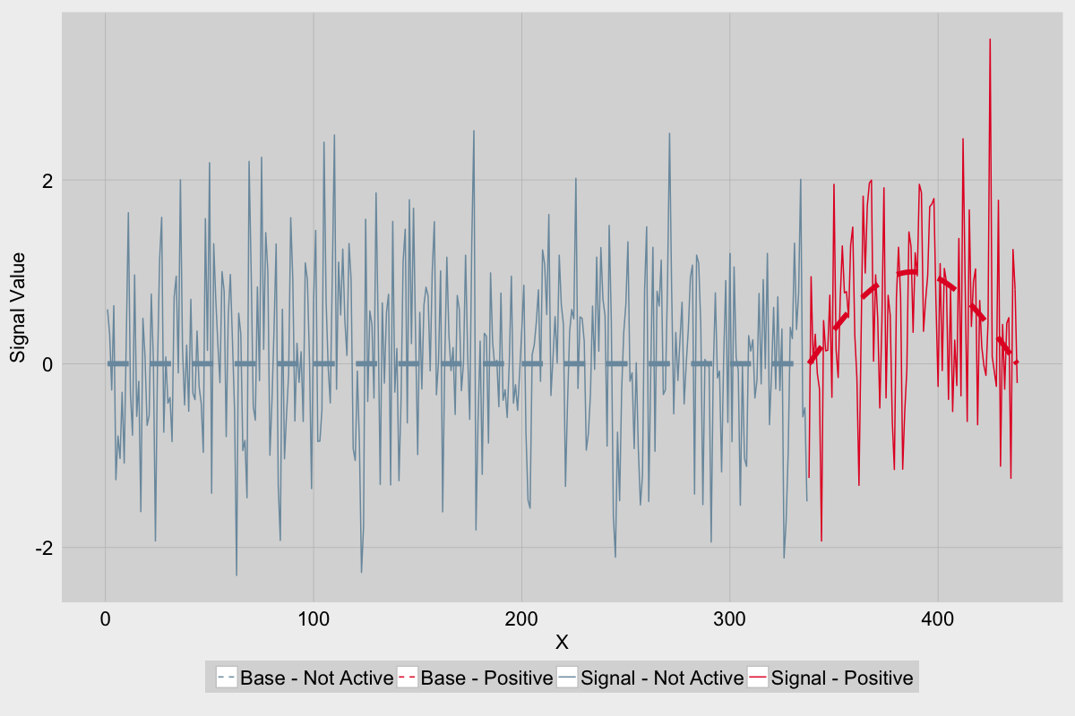
An example of one of the signals is shown below. The dashed line represents the base template for the signal which is a period of inactivity with a value of zero, followed by half a sine wave which represents positive activity. The solid lines represent the signal which is a combination of the baseline signal and random noise. The color blue represents the period of inactivity while the red portion is the area of positive activity.

To detect the positive activity I will be implementing a simple CUSUM test. CUSUM uses a cumulative sum to track changes between the signal and a reference signal. For this example I will use the mean of the signal as the reference. At each sample the distance from the mean is calculated and added to the cumulative sum calculated in the previous sample. If the new cumulative sum is not positive, then the cumulative sum is reset to zero. The function below is used to calculate the cumulative sum for each sample.

get_cumulative_sum <- function(y, reference){
  n <- length(y)
  # s - cumulative sum 
  s <- rep(0,n)
  if(n==1){
    return(s)
  }
  s <- rep(0,n)
  for(i in 2:n){
    s[i] <- max(0,s[(i-1)] + y[i]-reference[i]) 
  }
  return(s)
}

The next step is to create the test set which is comprised of 100 signals containing the following attributes:

x - The index of sample. When using real time series data this would be the time/date value.
y - Amplitude of the signal.
y.noise.removed - The base signal without noise.
positive.activity
- 1 - positive activity
- 0 - not active
s - The cumulative sum value
reference - The mean of the signal from the 1st y value to the current y value.

# create dataset of multiple different spikes
ids <- 1:100
ds  <- NULL
x.range   <- 1:1000
spike.length <- 100
for(ID in ids){
  g <- generate_spike(x.range,spike.length)
  x <- g$x
  y <- g$y
  y.noise.removed <- g$y.base
  positive.activity <- g$positive.activity
  reference <- cumsum(y)/seq_along(y)
  s <- get_s(y, reference)
  temp <- data.frame(ID,x,y,reference,s,
                     positive.activity, 
                     y.noise.removed)
  ds <- rbind(ds, temp)
}

To perform AMOC analysis a scoring function must be set up. In this example I will use the following scoring rules:

1 - Event detected in the first 100 samples of positive activity
0 - All other outcomes

You will note the spike generator function always ends with 100 samples of positive activity. When using AMOC, each individual test should end with the area of positive activity cut off at the desired period of detection. For example if I want to detect an alert within 5 hours of the onset of positive activity, then the test will be carried out on the signal from the 1st sample up until 5 hours after the onset of positive activity.

A false alarm is defined as any event detected prior to the onset of positive activity.

thresholds <- seq(-20,120,0.5)
final.scores <-NULL
# score function 
# 1 - alarm triggered within 100 samples of the onset of positive
#   activity
# 0 - all other scenarios
for(t in thresholds){
  scoring.results <- ds %>% group_by(ID) %>%
    transmute(
       event.detected = s>t,
       false.alarm = event.detected & positive.activity == 0,
       score       = event.detected & positive.activity ==1
      )
  score.stats <- scoring.results %>% group_by(ID) %>%
    summarise(
      score = max(score),
      f.sum = sum(false.alarm),
      n.samples = n() - spike.length
    )
  false.alarm.rate <- sum(score.stats$f.sum)/sum(score.stats$n.samples)
  total.score      <- mean(score.stats$score)
  final.scores <- rbind(final.scores,
                        data.frame(threshold = t,
                                   false.alarm.rate,
                                   total.score))
}

Note in the code above that the score does not take into account redundant warnings. In most cases, if we are detecting an event it is irrelevant that the event is detected again after the initial alert. However we could adjust the scoring mechanism to weight the score based on how fast an event is detected.

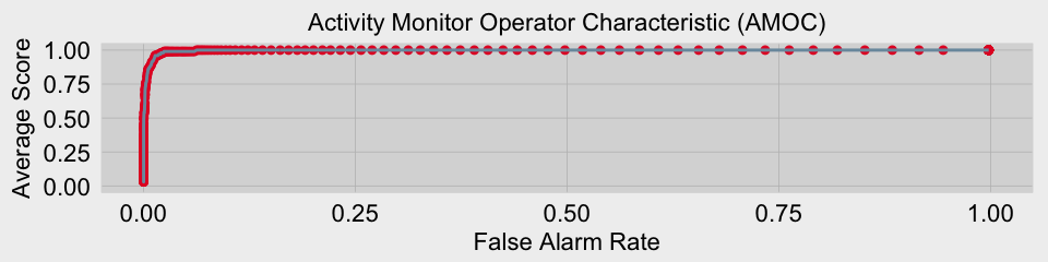
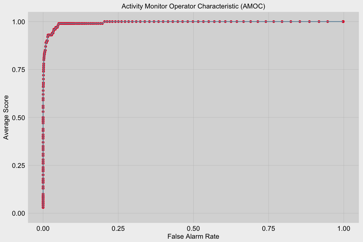
The last step is to create the AMOC curve.

final.score.plot <- ggplot(final.scores, aes(x = false.alarm.rate, y = total.score)) +
  scale_x_continuous(limits = c(0,1), breaks = seq(0,1,0.25)) +
  scale_y_continuous(limits = c(0,1), breaks = seq(0,1,0.25)) + 
  labs(x = "False Alarm Rate", y = "Average Score",
       title = "Activity Monitor Operator Characteristic (AMOC)") +
  geom_point(color = "#E4002B", size = 3) + 
  geom_line(color = "#7A99AC", size = 1)

The AMOC curve is shown below. We now have a measure of how well the event detector works independent of the threshold used for detection.

Below are links to the paper by Fawcett and Provost as well as tutorial slides on event detection by Neil and Wong.

¹T. Fawcett and F. Provost, “Activity monitoring: Noticing interesting changes in behavior,” Proc. fifth ACM SIGKDD Int. Conf. Knowl. Discov. data Min., vol. 1, no. 212, pp. 53–62, 1999.