Overview
When analyzing a time series some common questions are:
- What is the overall trend of the data?
- Does the output change with season? (quarterly, daily, monthly, etc.)
However these answers are often not easily observable due to noise present in the data. One of the tools which can be used to remove noise, isolate the overall trend, and identify any seasonal characteristics is time series decomposition using moving averages. To help explain this method I will use open data on Philadelphia crime incidences from 2012-2014 available at opendataphilly. You can also take a look at my dashboard app which provides time series decompositions for each type of crime in the dataset as well as an interactive map.
Moving on to time series decomposition…
Step 1: Identify the Type of Model
The first step is determining if the model is additive or multiplicative. Additive models can be identified as having a relatively stable frequency over time. An example of an additive model is provided below.
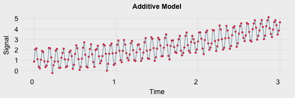
An additive model can be described using the following equation:
Y[t] = T[t] + S[t] + e[t]
- Y[t] : Output of the model
- T[t] : Trend component of the model
- S[t] : Seasonal component of the model
- e[t] : Noise/remainder
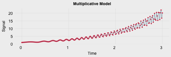
Multiplicative models exhibit a change in frequency over time and are described using the following equation:
Y[t] = T[t] * S[t] * e[t]
An example of a multiplicative model is shown below. Note there is an increasing trend which is also accompanied by an increase in frequency over time.
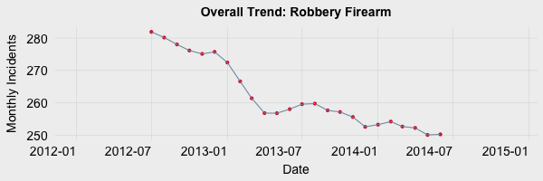
Philadelphia’s Robbery via Firearm crime data, as well as nearly all other crime types, can be described using an additive model as the seasonal variations remain relatively constant over time. The remainder of this post will focus on decomposition using the additive model.
Step 2: Identify the Trend
The trend component of a time series is identified using a moving average filter. I’ve decided to look at the data in terms of monthly incident counts. Since there are 12 months in a year I need to use a moving average of length twelve. This means that at each point I want to average the 6 steps behind and 6 steps in front of the position I am calculating an average value for. However since my moving average is an even length I have to take the average of two averages as shown in the graphic below.
We begin taking moving averages at position 7 in the data since this is the first position with 6 trailing values. To calculate the moving average of position 7, I first take the average of elements 1 through 12. Then I take the average of positions 2 through 13. These two averages are then averaged together to give me my moving average for position 7.
The moving average is calculated for each element from element 7 until there are no longer 6 leading values remaining. Below is an example of the sliding window for the moving average. Each time it advances to the next element, the whole window shifts. In the case of element 7 we required elements 1 through 13 to calculate our moving average. The average for element 8 will use 2 through 14, element 9 will use 3 through 15, and so on.
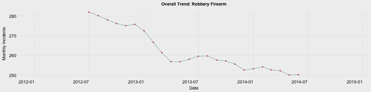
The result of these moving averages yeilds the overall trend of the data. The trend plot representing Robberies via Firearm from 2012 to 2014 are shown in the graph below. Note the six month lag and six month lead on each end of the trend. This is due to the moving average which needs 6 months of data both behind and in front of each month’s data to calculate the average.
One last note on moving averages: if there were 13 months in a year, only one average would need to be taken at each position as opposed to the average of two averages. This is due to the fact that a center value exists when the window is an odd number of elements (6 lag, current element, 6 lead).
Step 3: Identify Seasonal Component
The seasonal component of the time series is found by subtracting the trend component from the original data then grouping the results by month and averaging them. Below is some basic R code to describe this process. The montly incident count, event, and the previously calculated trend values are stored in a dataframe entitled monthly.incidents. I use dplyr to group the counts by month, subtract the trend from the number of events, then take the average for that given month. After the average for each month has been calculated, the seasonal trend value for each month is normalized by subtracting the mean of all avg.seasonal values from each individual avg.seasonal value.
# first ten entries of the montly incidents table
General.Crime.Category events    trend  month
                   (fctr)  (int)    (dbl) (fctr)
1         Robbery Firearm    282       NA    Jan
2         Robbery Firearm    226       NA    Feb
3         Robbery Firearm    216       NA    Mar
4         Robbery Firearm    239       NA    Apr
5         Robbery Firearm    291       NA    May
6         Robbery Firearm    247       NA    Jun
7         Robbery Firearm    314 281.9167    Jul
8         Robbery Firearm    314 280.1667    Aug
9         Robbery Firearm    342 278.0417    Sep
10        Robbery Firearm    313 276.1667    Oct

monthly.incidents %>% group_by(month) %>%
  summarise(
    avg.seasonal = mean(events - trend, na.rm = T)
  ) %>% mutate(
    normalized.seasonal = avg.seasonal-mean(avg.seasonal)
  )

    month avg.seasonal normalized.seasonal
   (fctr)        (dbl)               (dbl)
1     Jan    22.145833           20.454861
2     Feb   -77.416667          -79.107639
3     Mar   -74.041667          -75.732639
4     Apr   -33.541667          -35.232639
5     May    12.062500           10.371528
6     Jun    -3.145833           -4.836806
7     Jul    -5.250000           -6.940972
8     Aug    22.541667           20.850694
9     Sep    33.145833           31.454861
10    Oct    32.333333           30.642361
11    Nov    54.125000           52.434028
12    Dec    37.333333           35.642361
The normalized seasonal trend for Robberies via Firearm is shown below.
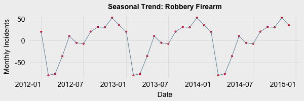
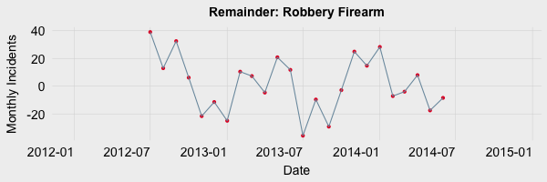
Step 4: Identify Noise/Irregularity
The noise component, also reffered to as the irregular or random component, is composed of all the leftover signal which is not explained by the combination of the trend and seasonal component. To quantify this component the trend and seasonal components are subtracted from the original signal (no averages or filtering, just subtraction). The noise component in the Robberies via Firearm data is shown below.
Summary
Time series decomposition using moving averages is a fast way to view seasonal and overall trends in time series data. There are a variety of different methods for processing and analyzing time series, but this is a good starting point. If you are interested in performing time series analysis, the decompose function in R provides the seasonal, trend, and noise components for both additive and multiplicative models as covered in this post.