Overview

Philadelphia has an abundance of open data which can be found on the Open Data Philly website. I decided to take a look at the crime data from 2006 through 2014 and create a Shiny app, which you can view here, to visualize the data. The rest of this post will highlight only certain portions of the code, but the complete code for the app can be found here.

Yearly Crime Trend

My first step in exploring the data was to create a yearly crime trend plot. The goal was to create a trend plot based on two user inputs: crime type and year the crime occurred. I imported all the 2006-2014 csv files using RCurl then combined them into a single dataframe. From this point I am left with a dataframe, ds, which contains information about each incident. I narrow down this information into the number of incidents on each individual day grouped by crime type, the column labeled TEXT_GENERAL_CODE. Below is the code which uses functions from the dplyr and lubridate packages.

#ds contains 2006-2014 crime data

# convert to date and times using lubridate
ds$DISPATCH_DATE <- ymd(ds$DISPATCH_DATE)
ds$DISPATCH_TIME <- hms(ds$DISPATCH_TIME)


# remove the space from 'homicide - criminal '
ds$TEXT_GENERAL_CODE <- as.character(ds$TEXT_GENERAL_CODE)
ds$TEXT_GENERAL_CODE[ds$TEXT_GENERAL_CODE == "Homicide - Criminal "] <- 
  "Homicide - Criminal"
ds$TEXT_GENERAL_CODE <- as.factor(ds$TEXT_GENERAL_CODE)

# get monthly counts split by individual date and crime type
event.log <- ds %>% group_by(DISPATCH_DATE, TEXT_GENERAL_CODE) %>%
  summarise(
    event.count = n()
  )

# get the year, month, and day of the year for the dispatch date
event.log$year <- year(event.log$DISPATCH_DATE)
event.log$month <- month(event.log$DISPATCH_DATE)
event.log$yday   <- yday(event.log$DISPATCH_DATE)

I originally split the data by day and crime type so that I could look at a variety of temporal trends, but for now I will focus on the monthly incident counts. Therefore to create the plot I need to filter the data for the selected crime type and year. To create the plot I will use ggplot2 as shown below. The app contains two input selectors for crime type, input$crime.type and year, input$year.

# filter the event log and 
# calculate monthly incident counts
  data <- filter(event.log, 
                     TEXT_GENERAL_CODE == input$crime.type & 
                       year %in% input$year) %>%
                       group_by(month,year) %>%
                       summarise(
                         monthly.count = sum(event.count)
                       )

  ggplot(data, 
         aes(x = month, y = monthly.count, color = factor(year))) +
    stat_smooth(se = F) + geom_point() + 
    scale_color_brewer(palette="Set1",
                       name = "Year") + 
      labs(title = paste('Philadelphia Crime Occurences:', input$crime.type),
           x = "", y = "Occurrences") + 
    scale_x_continuous(breaks = 1:12, labels = month(1:12, label = T) ) +
    fte_theme()

The resulting crime trend plot is shown in the animation below.

Mapping Crime with Leaflet

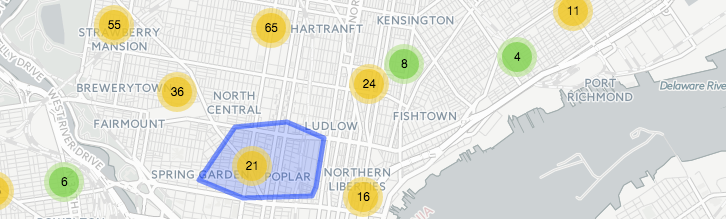
The second visualization is a map built using the leaflet package which is essentially a wrapper for leaflet.js. Similar to the crime trend graph, I want to show the incidents based on the user selected crime type and year. I use the filter function from dplyr to select the requested data. The leaflet() function creates a map widget. Then I add the base map tile layer to the map widget using the addProviderTiles() function. I selected a third-party base map, CartoDB.Positron, but many others options are available here. To set the level of zoom and the center coordinates of the map, the setView() function is used. The final step is to add the markers for each incident to the map. However I have a very large number of incidents to map, so I elected to use the leaflet cluster plugin which allows markers which are close to one another to be grouped together. When clicking on a cluster it zooms in to the clustered area and shows individual incidents.

points <- filter(coordinates, 
                     TEXT_GENERAL_CODE == input$crime.type.map & 
                       year %in% input$year.map)
    
    leaflet() %>%
      addProviderTiles('CartoDB.Positron') %>%
      setView(lng=-75.06048, lat=40.03566, zoom = 11) %>%
      addCircleMarkers( data = points,
                        lat = ~POINT_Y, lng = ~POINT_X,
                  clusterOptions = markerClusterOptions()
      )

The resulting map can be seen below.

Summary

I built this app as an exercise to learn how to use the leaflet package in R, but I find myself wanting to continue exploring the data. The following ideas come to mind:

Seasonal Trend Analysis: Does the rate of crime increase/decrease based on the time of year and/or location? Do these trends correlate with specific events?
Crime Data Part II: Philadelphia released additional crime data on 10/1/2015 which provides times and locations of different types of crime not provided in the datasets I originally analyzed.

Please feel free to contact me via Twitter or Github if you would like to contribute or provide feedback in regards to this project.