What is it?

The normal distribution, also known as a Gaussian distribution, is a continuous probability distribution that describes a number of populations we see in everyday life. It is known for it’s bell shaped curve and has 3 primary properties (Urdan, T. (2010)):

1. Asymptotic: The tails of the distribution never go to zero, i.e. they never touch the x-axis
2. Mean, Median, and Mode are all at the same place in the center of the distribution.
3. Symmetric: The upper and lower tails are mirror images of one another.

What is a Probability Distribution?

A probability distribution is a list of all possible outcomes and their corresponding probabilities. (Kruschke, J. (2015))

What is it used for?

The normal distribution is used to model many events occurring in our world. In statistics we can use our knowledge of the normal distribution to calculate the probability of a random variable. For example, say I have a sample of adults and I want to know the probability of a random sample having a height between 60 and 62 inches. I can determine the probability using the normal distribution. This post will only focus on the general properties and parameters of the distribution. In upcoming posts I will go over the calculation of probability. In addition to estimation of probability, the normal distribution is also used as an integral part of many different statistical tests and machine learning applications.

It is extremely important to have an understanding of the normal distribution as you will often find that the ‘assumption of normality’ is being made by different methods. If this assumption is wrong you will need to change your course of action for the problem you are solving.

Terminology

Parameters:

Mean
Description: The mean is the parameter that signifies the centrality of the distribution.
Symbol: μ - Symbol Name: Mu

Standard Deviation
Description: The standard deviation determines the spread of the data. Another way to think about this is that the standard deviation determines how dense the probability is surrounding the mean. High standard deviation ~ probability is spread out across a wider range (less dense), low standard deviation ~ probability surrounding the mean is more dense.
Symbol: σ - Symbol Name: Sigma

Experiment with the interactive data visualization below to get a better sense of how the parameters effect the shape of the distribution:

Standard Normal Distribution

You will often see references to the standard normal distribution. It is the normal distribution with a mean of zero and a standard deviation of 1. When we want to calculate the probability of a random sample we will scale a normal distribution ,using the standard normal distribution, then derive the probability. This process is known as standardization and will be discussed in an upcoming post.

When Should I Use This?

Use:

In upcoming post I will go into detail on how we can use the normal distribution. For now, know that the normal distribution can be used to derive the probability of a random variable when it is originating from a normal distribution. In addition, it is used as an integral part in a variety of applications.

Don’t Use:

If you are working with data from a sample that is non-normal.

Assumptions, Prerequisites, and Pitfalls

If you are unsure of the distribution your data was drawn from do not automatically assume it was from a normal distribution. If you assume normality incorrectly any results you derive cannot be trusted. It is always best to test for normality if you are unsure.

Example - No Code

The ‘no-code’ example is an attempt to explain what probability density is. In this example we will use an example that we assume has a normal distribution.
How many ounces are actually in your pint glass when you order a beer?

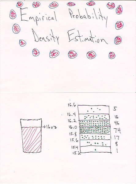
We recorded the number of ounces in 167 pours and plotted it in the histogram below.

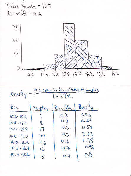
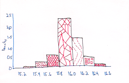
The probability density is the probability divided by the size of the bin. In our case the bin size is 0.2 ounces.

You may have noticed a couple of things in the example above:

1. Probability density can have a value greater than 1. Remember it is the density of probability in the bin, not a probability value.
2. We used bins with a width of 0.2 ounces to look at the density, but what would happen if I wanted to estimate the probability of a single point? In a continuous distribution there are infinite possible values and therefore the probability would approach zero. When we want to identify a probability for a specific value we have to use an interval (more on this in upcoming posts).

Example - Code

For the following examples I’ll work through some code examples of how the parameters, μ and σ, effect the shape of our distributions by plotting them in R and Python.

Python & Matplotlib

import numpy as np
from scipy.stats import norm
import matplotlib.pyplot as plt

# plot density using different parameters
x = np.linspace(-15,15, 1000)
params = [[1,1], [1,3], [3,1], [3,3]]
for p in params:
    value = norm.pdf(x,loc = p[0], scale = p[1])
    plt.figure(figsize=(8,2), dpi=72)
    plt.title(r'$\mu$' + ' = ' + str(p[0]) + ', ' + r'$\sigma$' +
                ' = ' + str(p[1]))
    plt.plot(x,value)
    plt.subplots_adjust(top=0.8)
    plt.savefig('nd_mean'+str(p[0])+'_sd'+str(p[1])+'_py.svg', format='svg')
    # clear figure
    plt.clf()

R & ggplot2

library(ggplot2)

n <- seq(-15,15,0.01)
mean_param <-c(0, 3)
sd_param   <-c(1,3)
params <- expand.grid(mean_param, sd_param)
names(params) <- c('mean', 'std')
for(i in 1:nrow(params)){
  ds <- data.frame(value = n, probability = dnorm(n,params[i,1],params[i,2]))

  p <- ggplot(ds, aes(x = value, y = probability )) +
    geom_density(stat='identity',                                                               fill='#0B6C8C') +
    labs(title =bquote(mu == .(params[i,1]) ~~ sigma == .(params[i,2])),
         x='x', y='p(x)')
  print(p)
}

References

^{Kruschke, J. (2015). Doing Bayesian data analysis : a tutorial with R, JAGS, and Stan. Boston: Academic Press.
Urdan, T. (2010). Statistics in plain English. New York: Routledge.}