2 Parameter Estimation

LDA is a generative probabilistic model, so to understand exactly how this works we need to understand the underlying probability distributions. In this chapter we will focus on the Bernoulli distribution and the Beta distribution. Both of these distributions are very closely related to (and also special cases of) the multinomial and Dirichlet distributions utilized by LDA, but they are a bit easier to comprehend. Once we have made our way through Bernoulli and beta, we will go over how they are linked to the multinomial and Dirichlet distributions.

Throughout the chapter I’m going to build off of a simple example - a single coin flip.

2.1 Distributions

2.1.1 Bernoulli

When you flip a coin you get either heads or tails as an outcome (barring the possibility it lands on it’s side). This single coin flip is an example of a Bernoulli trial and we can use the Bernoulli distribution to calculate the probability of either outcome. Any single trial with two possible outcomes can be modeled as a Bernoulli trial: team wins/loses, pitch is a strike/ball, coin comes up heads or tails, etc.

2.1.1.1 Bernoulli: A Special Case of the Binomial Distribution

You will often see Bernoulli distribution mentioned as a special case of the Binomial distribution. The binomial model consists of n Bernoulli trials, where each trial is independent and the probability of success does not change between trials.(Kerns 2010) The Bernoulli distribution is the case of a single trial (n=1).

I will use the term success interchangably with the term heads when describing Bernoulli distribution. In reality success could be tails if you choose to define it that way.

To clarify, if I want to calculate the probability of getting heads on a single coin flip I will use a bernoulli distribution. However, if I want to know the probability of getting 2 heads (or more) in a row, we would use the binomial distribution. For our purposes we are only concerned about the outcome of a single coin flip and will therefore stick to the Bernoulli distribution.

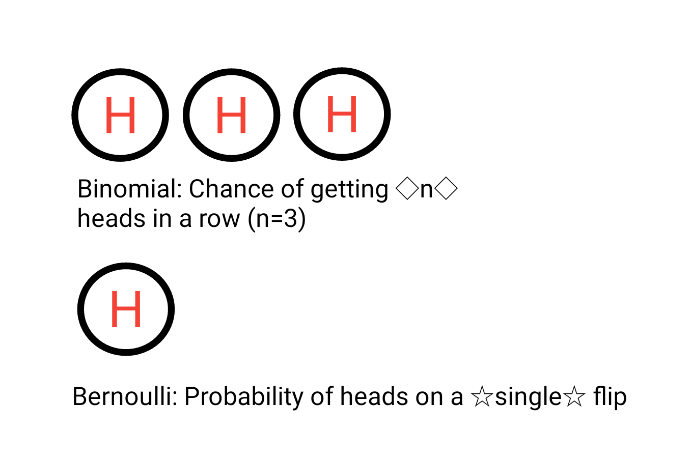
Figure 2.1: Bernoulli and Binomial Distributions

2.1.1.2 Bernoulli - Distribution Notation

The probability mass function of the bernoulli distribution is shown in Equation (2.1).

\[ \begin{equation} f_{x}(x)=P(X=x)=\theta^{x}(1-\theta)^{1-x}, \hspace{1cm} x = \{0,1\} \tag{2.1} \end{equation} \]

The only parameter of the bernoulli distribution is \(\theta\), which defines the probability of success during a bernoulli trial. The value of x is 0 for a failure and 1 for a success. In a practical example you can think of this as 0 for tails and 1 for heads during a coin flip. (2.2) is an example where the value of \(\theta\) is set to 0.7. We can see the probability of getting a success is 0.7, while the probability of failure is 0.3.

\[ \begin{equation} \begin{aligned} P(X=1)&=\theta^{1}(1-\theta)^{1-1}, \hspace{1cm} \theta=0.7 \\ P(X=1)&=0.7*1=0.7 \\\\ P(X=0)&=0.7^{0}(1-0.7)^{1-0}\\ P(X=0)&=0.3 \end{aligned} \tag{2.2} \end{equation} \]

2.1.2 Beta Distribution

The beta distribution can be thought of as a probability distribution of probabilities (Robinson 2014). The Bernoulli distribution is a distribution that gives us a probability of success (coin comes up heads). The beta distribution provides a distribution of these probabilities. To clear this up we will be working through some examples.

If you flip a coin 2 times resulting in 1 heads and 1 tails how sure are you that the coin is fair? Probably not all that sure. But what if you flipped the coin 200 times and it resulted in 100 heads and 100 tails? You would be much more confident that the coin is fair. The beta distribution gives us a way to quantify the probabilities (our confidence in the coin being fair).

The beta distribution has 2 shape parameters, \(\alpha\) and \(\beta\). These can be thought of as the results from the coin flips we just talked about (i.e. \(\alpha=200\), \(\beta=200\)). Below the probability density for different values of \(\theta\) is displayed based on different values of \(\alpha\) and \(\beta\). In general, the higher the value of \(\alpha\) and \(\beta\) the narrower the density curve is. Another way to think of this is that the more information (coin flip results) we have, the more confident we can be in our coin’s bias value (i.e. is it fair, head heavy, etc.).

a <- c(1, 10, 100)
b <- c(1, 10, 100)
params <- cbind(a,b)
ds <- NULL
n <- seq(0,1,0.01)
for(i in 1:nrow(params)){
  ds <- rbind(data.frame(x = n, y = dbeta(n, params[i,1], params[i,2]),
                             parameters = paste0("\U03B1 = ",params[i,1],
                                                 ", \U03B2 = ", params[i,2])), ds)
}

ggplot(ds, aes(x = x, y = y, color=parameters)) + geom_line() + 
  labs(x = '\U03B8', y = 'Probability Density') +
  scale_color_discrete(name=NULL) + theme_minimal()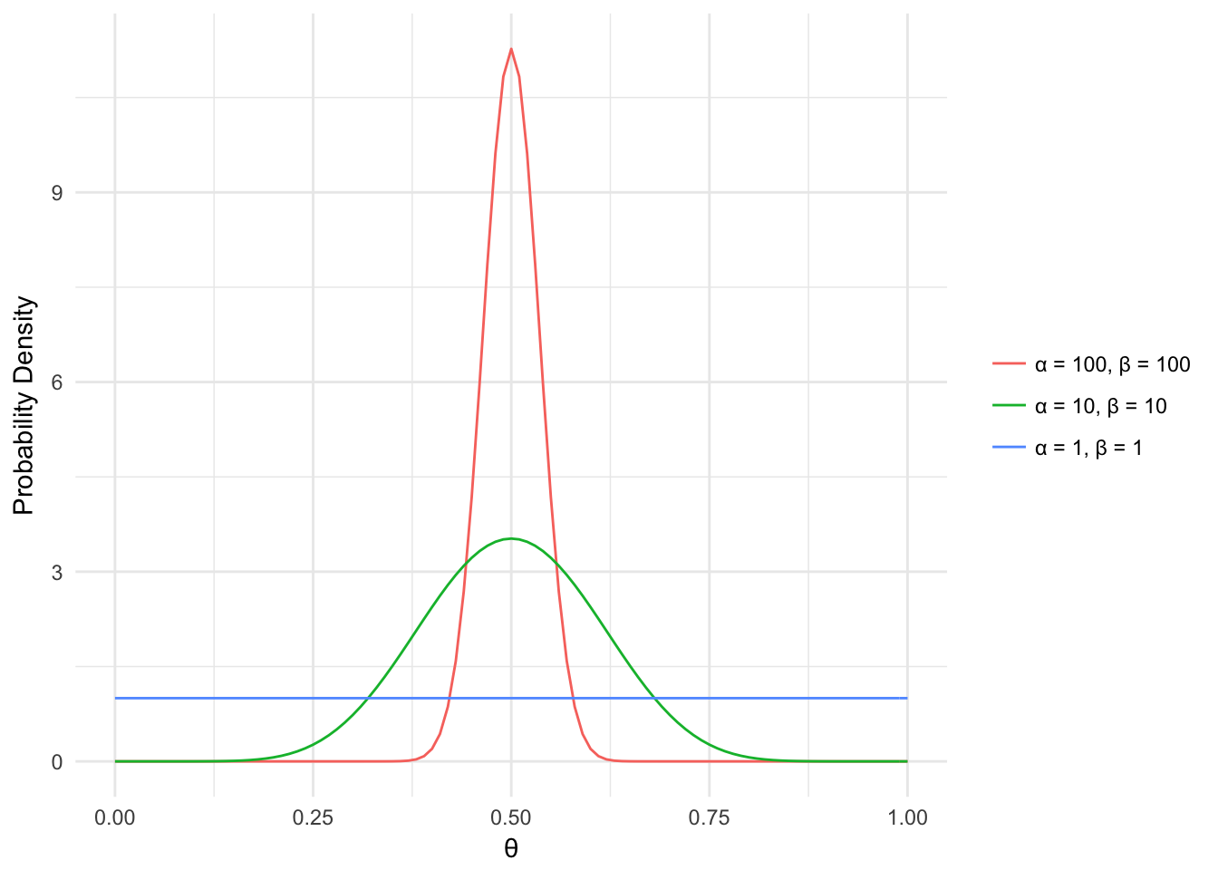

Figure 2.2: Beta Distribution

What about the cases where \(\alpha\) and \(\beta\) are not equal or close to equal? In those cases you would probably assume a bit of skew in the distribution, i.e. your coin may be biased toward head (density skewed toward 1) or tails (density skewed toward 0) as shown below.

a <- c(8, 2)
b <- c(2, 8)
params <- cbind(a,b)
ds <- NULL
n <- seq(0,1,0.01)
for(i in 1:nrow(params)){
  ds <- rbind(data.frame(x = n, y = dbeta(n, params[i,1], params[i,2]),
                             parameters = paste0("\U03B1 = ",params[i,1],
                                                 ", \U03B2 = ", params[i,2])), ds)
}

ggplot(ds, aes(x = x, y = y, color=parameters)) + geom_line() + 
  labs(x = '\U03B8', y = 'Probability Density') +
  scale_color_manual(name=NULL, values = c("#7A99AC", "#E4002B")) + theme_minimal()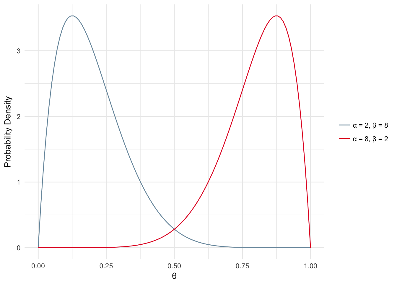

Figure 2.3: Beta Distribution - Skewed

The probability distribution function for the beta distribution can be found in Equation (2.3).

\[ \begin{equation} f(\theta;\alpha,\beta) ={{\theta^{(\alpha-1)}(1-\theta)^{(\beta-1)}}\over B(\alpha,\beta)} \tag{2.3} \end{equation} \]

• The Beta function, B is the ratio of the product of the Gamma function, \(\Gamma\), of each parameter divided by the Gamma function of the sum of the parameters. The Beta function is not the same as the beta distribution. The Beta function is shown below along with the Gamma function, which is used in the Beta function.

\[ \begin{equation} \beta(a,b) = {\Gamma(a)\Gamma(b) \over{\Gamma(a+b)}} \tag{2.4} \end{equation} \]

The Gamma function is the factorial of the parameter minus 1.

\[ \begin{equation} \Gamma(a) = (a-1)! \tag{2.5} \end{equation} \]

2.2 Inference: The Building Blocks

Equation (2.6) is a fundamental to understanding parameter estimation and inference.

\[ \begin{equation} \underbrace{p(\theta|D)}_{posterior} = {\overbrace{p(D|\theta)}^{likelihood} \overbrace{p(\theta)}^{prior} \over \underbrace{p(D)}_{evidence}} \tag{2.6} \end{equation} \]

The 4 components are:

• Prior: The probability of the parameter(s). Defines our prior beliefs of the parameter. Do we believe to a good degree of certainty that the coin is fair? Maybe take a step back and ask yourself ‘do I trust the manufacturer of this coin?’. If this manufacturer has always had great quality (i.e. fair coins) then you would have confidence your coin is fair. If you know nothing about where the coin came from you would be more skeptical of the coin’s bias.
  
• Posterior: The probability of the parameter given the evidence. Think of it this way, given 100 coin flips with 47 heads and 53 tails what is the probability that theta is 0.5 (coin is fair)? The only way to know this value is if you already obtained the evidence. However we can estimate the posterior in various ways some of which will be covered in this chapter.
• Likelihood: The probability of the evidence given the parameter. Given that we know the coin is fair (theta = 0.5) what is the probability of having 47 heads out of 100 flips?
• Evidence: The probability of all possible outcomes. Probability of 1/100 heads, 2/100 heads, …, 100/100 heads.

Conditioning your brain for LDA : We are starting with a coin flip, but the eventual goal is to link this back to words appearing in a document. Try to keep in mind that we think of a word similar to the outcome of a coin: a word exists in the document (heads!) or a word doesn’t exist in the document (tails!).

2.3 Maximum Likelihood

The simplest method of parameter estimation is the maximum likelihood (ML) method. Effectively we calculate the parameter (\(\theta\)) that maximizes the likelihood.

\[ \begin{equation} \underbrace{p(\theta|D)}_{posterior} = {\overbrace{\bf \Large p(D|\theta)}^{\bf \Large LIKELIHOOD} \overbrace{p(\theta)}^{prior} \over \underbrace{p(D)}_{evidence}} \tag{2.7} \end{equation} \]

Let’s first discuss what the likelihood is. The likelihood can be described as the probability of getting observed data given a specified value of the parameter, \(\theta\). For example, let’s say I’ve flipped a coin 10 times and got 5 heads, 5 tails. Assuming the coin is fair, \(\theta\) equals 0.5, what is the likelihood of observing 5 heads and 5 tails.

To calculate the likelihood of a parameter given an outcome we would use the probability mass function in Equation (2.8).

\[ \begin{equation} P(X=x)=\theta^{x}(1-\theta)^{1-x}, \hspace{1cm} x = \{0,1\} \tag{2.8} \end{equation} \] Where an outcome, x, of heads equals 1 and an outcome of tails is 0. Now let’s say we have carried out 10 coin flips:

\[ \begin{equation} \begin{aligned} P(X_{1}=x_{1},X_{2}=x_{2},...,X_{10}=x_{10}) &= \prod\limits_{n=1}^{10} \theta^{x}(1-\theta)^{1-x}\\ L(\theta) &= \prod\limits_{n=1}^{10} \theta^{x}(1-\theta)^{1-x} \end{aligned} \tag{2.9} \end{equation} \]

What is shown in Equation (2.9) is the joint probability mass function. Each coin flip is independent so we calculate the product of the PMF’s for each trial. This is known as the likelihood function - the likelihood of a value of \(\theta\) given our observed data.

Back to the maximum likelihood….

Our goal is to find the value of \(\theta\) which maximizes the likelihood of the observed data. To derive the maximum likelihood we start by taking the log of the likelihood, \(\mathcal{L}\).

\[ \begin{equation} \begin{aligned} \mathcal{L} &= log \prod\limits_{n=1}^N \theta^{x}(1-\theta)^{1-x} \\\\ &= \sum\limits_{n=1}^N log(\theta^{x}(1-\theta)^{1-x}) \\\\ &= n^{(1)}log(\theta) + n^{(0)}log(1-\theta) \end{aligned} \tag{2.10} \end{equation} \]

Then differentiate with respect to \(\theta\):

\[ \begin{equation} {d\mathcal{L} \over d\theta} = {n^{(1)}\over \theta} - {n^{(0)}\over 1-\theta} \tag{2.11} \end{equation} \]

Then set the left side of the equation equal to zero and solve:

\[ \begin{equation} \begin{aligned} 0 &= {n^{(1)}\over \theta} - {n^{(0)}\over 1-\theta} \\ \\ {n^{(1)}\over\theta} &= {n^{(0)}\over 1-\theta} \\ \\ {n^{1} - \theta n^{1}} &= {\theta n^{0}} \\ \\ n^{(1)} &= \theta(n^{(1)} + n^{0}) \\ \\ \theta &= {n^{(1)} \over N} \end{aligned} \tag{2.12} \end{equation} \]

The value of \(\theta\) that maximizes the likelihood is the number of heads over the number of flips. The maximum likelihood value for 1 out of 10 flips equal to head up to 10 heads out of 10 flips is shown in Figure 2.4.

heads = 1:10
flips = 10
ds <- data.frame(heads, flips = rep(flips, length(heads)))
ds$theta <- ds$heads/ds$flips


ggplot(ds, aes(x = heads,
               y = theta)) + 
  geom_point(color ='#1520c1', size = 3) + 
  geom_linerange(aes(x=heads,
                     y=NULL, ymax=theta,
                     ymin=0)) +
  scale_x_continuous(breaks = seq(0,10,2), labels = seq(0,10,2)) + 
  labs(y='\U03B8', x="Number of Heads", title ="ML Parameter Estimation: 10 Bernoulli Trials") +
  theme(plot.title = element_text(hjust = 0.5)) + theme_minimal()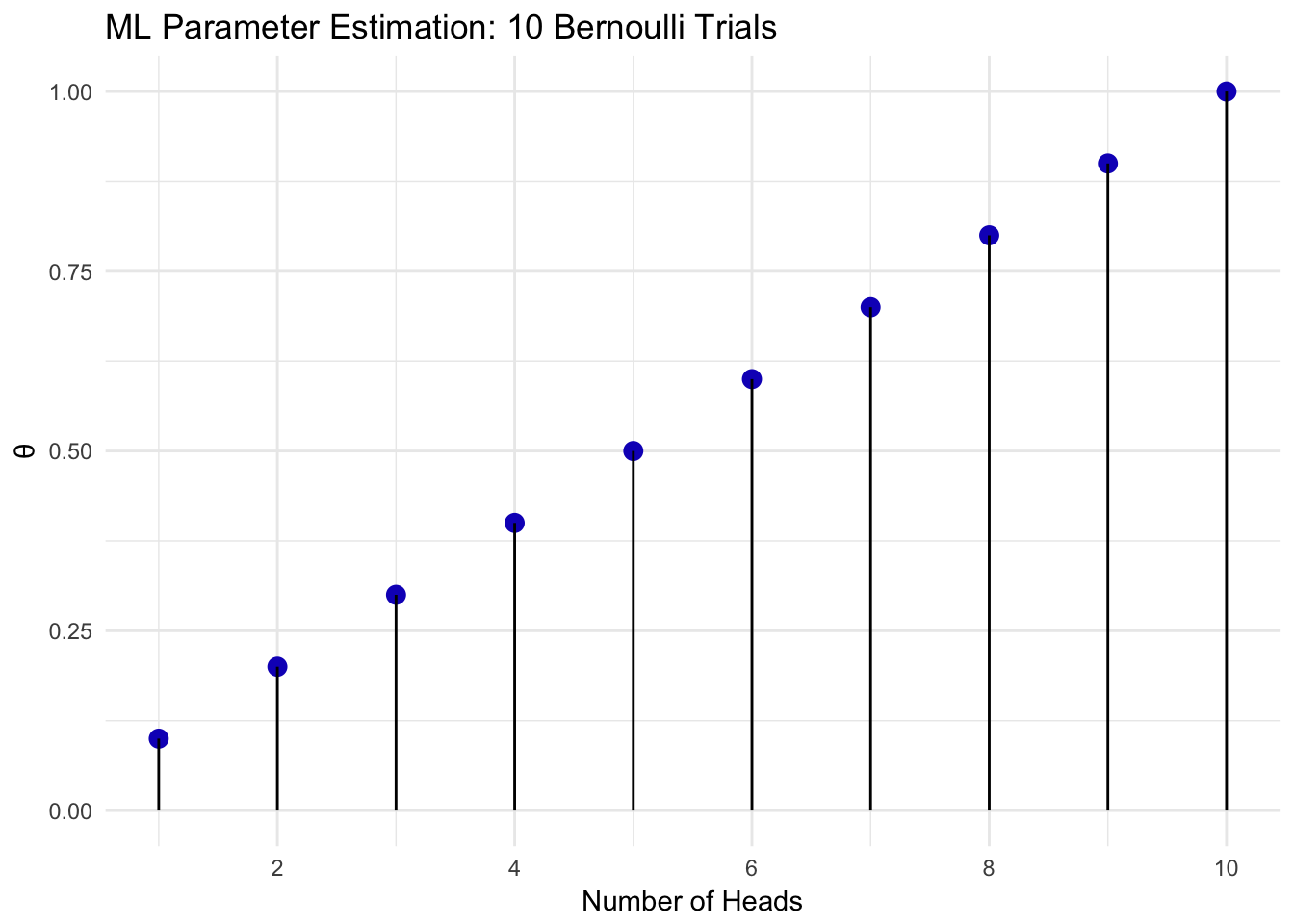

Figure 2.4: Bernoulli Maximum Likelihood

2.4 Maximum a Posteriori

Maximum a Posteriorir (MAP) is similar to the method of maximum likelihood estimation, but it also includes information about our prior beliefs. Unlike ML estimation, MAP estimates parameters by maximizing the posterior.

\[ \begin{equation} \theta_{MAP}=\underset{\theta}{\operatorname{argmax}} P(\theta|X) \tag{2.13} \end{equation} \]

\[ \begin{equation} \require{enclose} \theta_{MAP}=\underset{\theta}{\operatorname{argmax}}{\overbrace{p(D|\theta)}^{likelihood} \overbrace{p(\theta)}^{prior} \over \underbrace{\enclose{horizontalstrike}{p(D)}}_{evidence}} \tag{2.14} \end{equation} \]

The formula for the MAP estimation of \(\theta\) is shown in (2.14). The evidence term is dropped during the calculation of \(\theta_{MAP}\) since it is not a function of \(\theta\) and our only concern is maximizing the posterior based on \(\theta\). Similar to calculating the ML estimate, the first step is to apply the log function to the remaining terms (Equation (2.15)).

\[ \begin{equation} \begin{aligned} \theta_{MAP} &=\underset{\theta}{\operatorname{argmax}}p(D|\theta)p(\theta) \\\\ &= \mathcal{L}(\theta|D) + log(p(\theta)) \end{aligned} \tag{2.15} \end{equation} \]

We have already derived the log likelihood during our derivation of the maximum likelihood, so let’s now focus on the prior. The prior for the Bernoulli distribution is the Beta distribution and can be used to describe \(p(\theta)\). The probability distribution function, PDF, for the Beta distribution is shown in Equation (2.16).

\[ \begin{equation} p(\theta|\alpha,\beta) = {\theta^{\alpha-1}(1-\theta)^{\beta-1}\over{B(\alpha, \beta)}} \tag{2.16} \end{equation} \]

Next, we plug in the PDF of the beta distribution in the place of the prior (Equation (2.17)).

\[ \begin{equation} \begin{aligned} \theta_{MAP}&= \mathcal{L}(\theta|D) + log(p(\theta)) \\\\ \theta_{MAP}&= n^{(1)}log(\theta) + n^{(0)}log(1-\theta) + log({\theta^{\alpha-1}(1-\theta)^{\beta-1}\over{B(\alpha, \beta)}}) \\\\ \theta_{MAP}&= n^{(1)}log(\theta) + n^{(0)}log(1-\theta) + \\ &\quad log({\theta^{\alpha-1}) + log((1-\theta)^{\beta-1}) - log({B(\alpha, \beta)}}) \\\\ {d \over d\theta} \mathcal{L}(\theta|D) + log(p(\theta)) &= {n^{(1)}\over \theta} - {n^{(0)}\over 1-\theta} + {\alpha - 1\over\theta} - {\beta - 1 \over 1-\theta} \\\\ 0 &= {n^{(1)}\over \theta} - {n^{(0)}\over 1-\theta} + {\alpha - 1\over\theta} - {\beta - 1 \over 1-\theta} \\\\ \theta_{MAP}&= {{n^{(1)} + \alpha -1} \over {n^{(1)} + n^{0} + \alpha + \beta - 2}} \end{aligned} \tag{2.17} \end{equation} \]

Now that we know how to calculate the parameter \(\theta\) that maximizes the posterior, lets take a look at how choices of different priors and different numbers of observed trials effects our outcome.

In the Figure 2.5 we see the MAP estimation of \(\theta\) with a relatively uninformed prior, low \(\alpha\) and \(\beta\) values and a small number of observed experiments (n=20). Uninformed means we are going to make a weak assumption about the prior. In more general terms, this means that we don’t have a strong intuition that our coin is fair or unfair. In a mathematical sense, uninformed means a low sum of the two parameters, if you had \(\alpha=1000\) and \(\beta=1\) this would not be considered as uninformed whereas \(\alpha\) and \(\beta\) both equal to 1 is normally referred to as uniformed or naive. The Beta distribution has \(\alpha\) and \(\beta\) parameters of 2 resulting in the blue density curve shown in Figure 2.5.

The terms weak, uninformed, and naive are often used interchangeably when referencing priors. The same goes for the terms strong and informed.

n <- 20
heads <- 14
tails <- 6


B <- 2
alpha <- 2

map_theta <- (heads + alpha - 1)/(heads + tails + alpha + B -2)
possible_theta <- seq(0,1,0.01)
beta_ds <- data.frame(theta = possible_theta, density = dbeta(possible_theta, alpha,B))
ggplot(beta_ds, aes(x = theta, y = density)) + geom_point(color='#7A99AC') + 
  geom_vline(xintercept=map_theta, color = '#ba0223') + 
  annotate("text", x = map_theta + 0.1, y=0.5, label= paste("\U03B8[MAP]==", round(map_theta,2)), parse=T)+
  labs(x='\U03B8') + theme_minimal()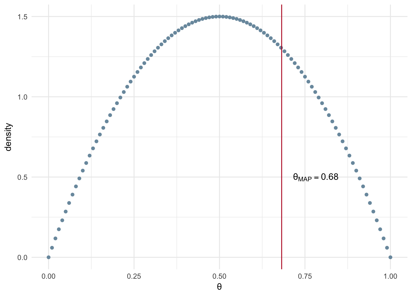

Figure 2.5: MAP: Small number of experiments and uninformed prior

In the next example we have the same number of samples, but we assume a much stronger prior. In particular, we assume the coin is most likely fair by selecting \(\alpha\) and \(\beta\) parameters both equal to 100. These parameters represent a Beta distribution that is centered at 0.5 and is very dense around that point. We can see the resuting MAP estimate is much closer to 0.5 than our previous example with the uniformed prior.

n <- 20
heads <- 14
tails <- 6

B <- 100
alpha <- 100

map_theta <- (heads + alpha - 1)/(heads + tails + alpha + B -2)
possible_theta <- seq(0,1,0.001)
beta_ds <- data.frame(theta = possible_theta, density = dbeta(possible_theta, alpha,B))
ggplot(beta_ds, aes(x = theta, y = density)) + geom_line(color='#7A99AC') + 
  geom_vline(xintercept=map_theta, color = '#ba0223') + 
  annotate("text", x = map_theta + 0.1, y=11, label= paste("\U03B8[MAP]==", round(map_theta,2)), parse=T)+
  labs(x='\U03B8', y = 'Density') + theme_minimal()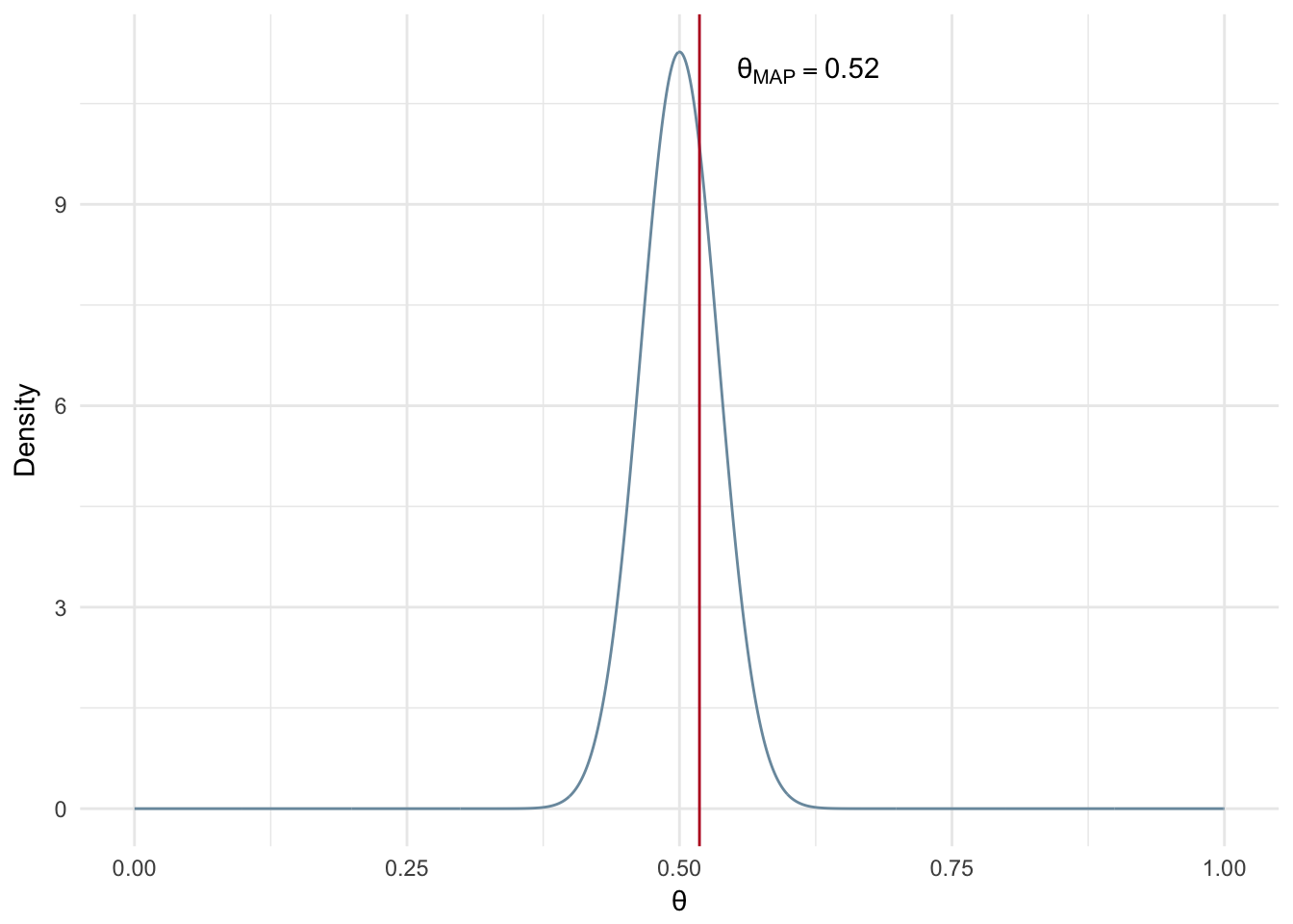

Figure 2.6: MAP: Small number of experiments and informed prior

What happens when we have a much larger number of observed experiments and an uninformed prior? In this case the MAP estimate will give us a value that is very close to a maximum likelihood estimate, i.e. heads divide by number of trials.

n <- 1000
heads <- 723
tails <- n-heads


B <- 2
alpha <- 2
map_theta <- (heads + alpha - 1)/(heads + tails + alpha + B -2)
possible_theta <- seq(0,1,0.001)
beta_ds <- data.frame(theta = possible_theta, density = dbeta(possible_theta, alpha,B))
ggplot(beta_ds, aes(x = theta, y = density)) + geom_line(color='#7A99AC') + 
  geom_vline(xintercept=map_theta, color = '#ba0223') + 
  annotate("text", x = map_theta + 0.1, y=1.2, label= paste("\U03B8[MAP]==", round(map_theta,2)), parse=T)+
  labs(x='\U03B8', y = 'Density') + theme_minimal()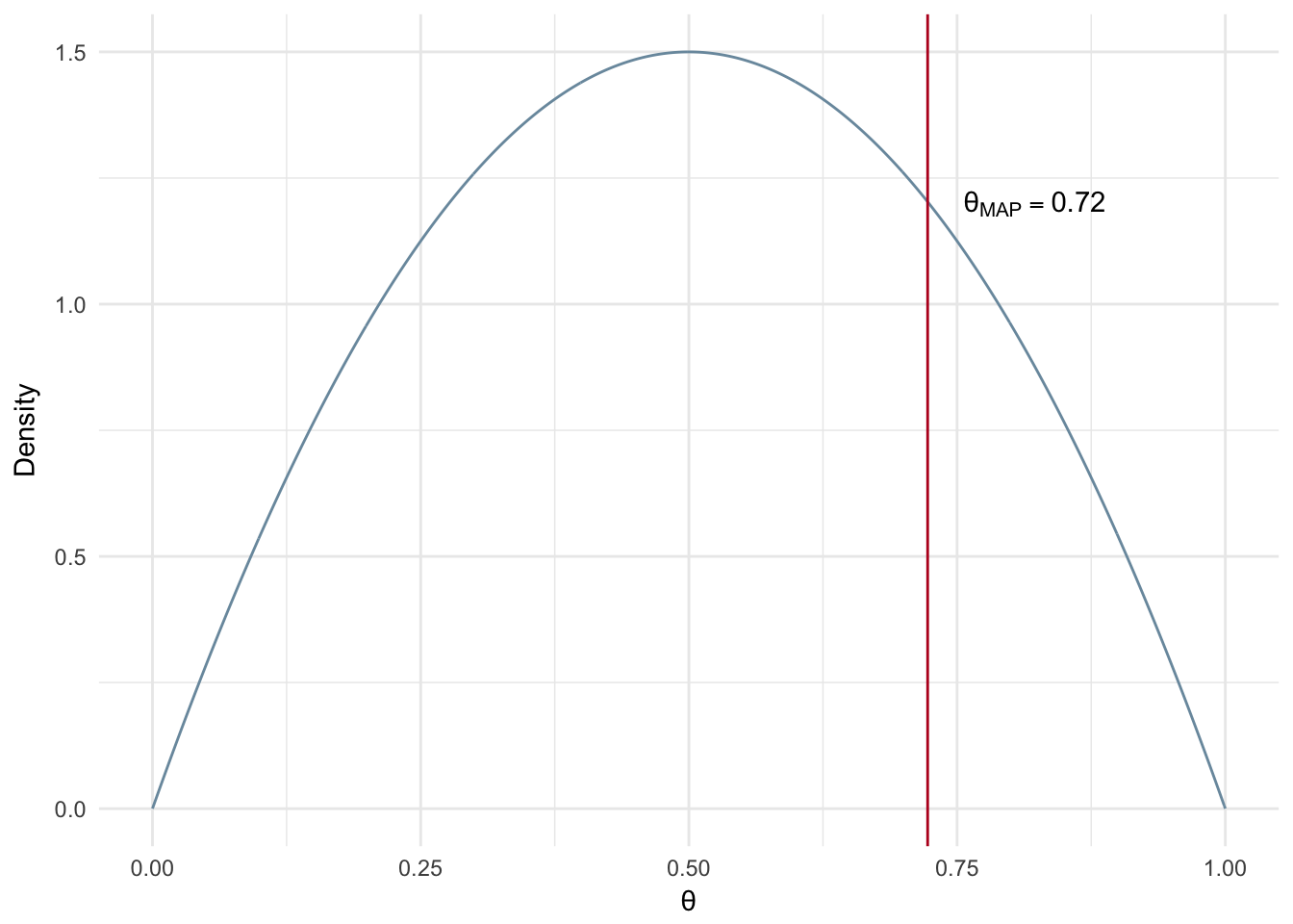

Figure 2.7: MAP: Large number of experiments and uninformed prior

Now let’s assume a much stronger prior, i.e. more confidence a priori the coin is fair, while using the same number of experiments. Notice that when we use a larger number of experiments it overpowers the strong prior and gives us a very similar MAP estimate in comparison to the example with the uninformed prior and the same number of experiments (Uninformed - Figure 2.7 and Informed - Figure 2.8).

n <- 1000
heads <- 723
tails <- n-heads

B <- 100
alpha <- 100
possible_theta <- seq(0,1,0.001)
beta_ds <- data.frame(theta = possible_theta, density = dbeta(possible_theta, alpha,B))
map_theta <- (heads + alpha - 1)/(heads + tails + alpha + B -2)
ggplot(beta_ds, aes(x = theta, y = density)) + 
  geom_line(color='#7A99AC') + 
  geom_vline(xintercept=map_theta, color = '#ba0223') + 
  annotate("text", x = map_theta + 0.1, y=8.2, label= paste("\U03B8[MAP]==", round(map_theta,2)), parse=T)+
  labs(x='\U03B8', y = 'Density') + theme_minimal()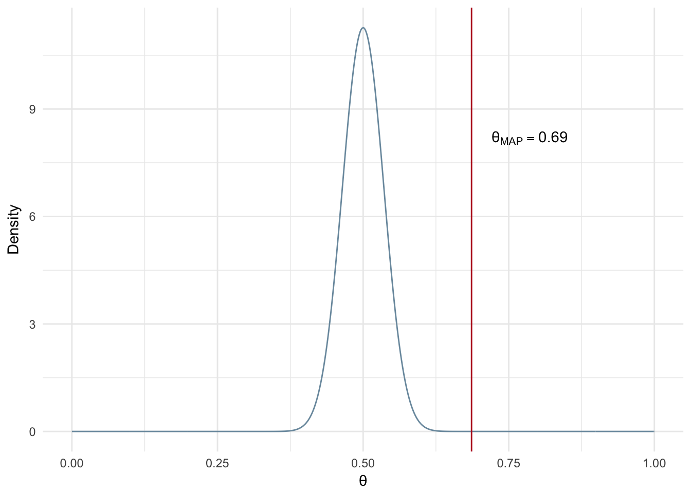

Figure 2.8: MAP: Large number of experiments and informed prior

In summary:

• The stronger your prior assumptions are, the more observations you will need to overcome an incorrect prior estimation/belief.
• Stronger prior - MAP estimate moves toward most dense area of prior distribution
• Weaker prior - MAP looks more like a maximum likelihood

2.5 Bayesian Inference

2.5.1 Analytical Solution

Another option we have for estimating parameters is to estimate the posterior of the distribution via Bayesian inference. In our MAP estimation example we included prior assumptions as part of our calculation. We are going to do the same via Bayesian inference however instead of a point estimate of \(\theta\), we will be calculating the posterior distribution over all possible values of \(\theta\). From this we can take the expected value of \(\theta\) as our estimated parameter.

In the case of the coin flip, Bayesian inference can be solved analytically. We have reviewed the likelihood and the prior, but when estimating the posterior we need to include the evidence term. This is somewhat tricky.

\[ \begin{equation} \underbrace{p(\theta|D)}_{posterior} = { p(D|\theta) p(\theta) \over \underbrace{p(D)}_{evidence}} \tag{2.18} \end{equation} \]

\[ \begin{equation} p(D) = \int_{\theta}p(D|\theta)p(\theta)d\theta \tag{2.19} \end{equation} \]

\[ \begin{equation} {p(\theta|z,N)} = {\overbrace{\theta^z(1-\theta)^{(N-z)}}^{likelihood} \overbrace{{\theta^{(a-1)}(1-\theta)^{(b-1)}}\over \beta(a,b)}^{prior}\over{\underbrace{\int_{0}^1 \theta^z(1-\theta)^{(N-z)}{{\theta^{(a-1)}(1-\theta)^{(b-1)}}\over \beta(a,b)}d\theta}_{Evidence}}} \tag{2.20} \end{equation} \]

In Equation (2.19) we see the evidence term is an integral over all values of \(\theta\), 0 to 1. This means the value is a constant. Recall that the evidence term acts as a scaling factor to ensure our probabilities sum to 1. We will plug in a generic placeholder of our evidence value in (2.21) since we have established that it is a constant.

\[ \begin{equation} \begin{aligned} p(\theta|z, N) &= {\theta^{z}(1-\theta)^{(N-z)}{{\theta^{(a-1)}(1-\theta)^{(b-1)}}\over \beta(a,b)}\over{C}} \\\\ &= {\theta^{(z+a-1)}(1-\theta)^{(N-z+b-1)} \over \beta(z+a, N-z+b)}\\\\ &= Beta(z+a, N-z+b) \end{aligned} \tag{2.21} \end{equation} \] In the second step of Equation @(eq:bernBIFinal) the beta function (the denomitor of the prior) takes the place of the constant (i.e. the evidence value). The beta function is a constant value and we need it to do the same job as the evidence term; it needs to ensure the probabilities sum to 1. To ensure this we alter the input parameters to the beta function, so that we are left with a beta distribution for our posterior that includes our observed experiments and our prior’s hyperparameters.

To estimate \(\theta\), we calculate the expected value of a Beta distribution as shown in Equation @(eq:bernBIExp).

\[ \begin{equation} E[\theta]={\alpha \over \alpha + \beta} \tag{2.22} \end{equation} \]

Plugging in our parameters, as per the derivation in Equation @(eq:bernBIFinal), we get the resulting expected value of \(\theta\) shown in @(eq:bernBIExpFinal)

\[ \begin{equation} \begin{aligned} E[\theta] &= {z+a \over {z+a + n-z+b}}\\\\ &={z+a \over {a+N+b}}\\\\ \end{aligned} \tag{2.23} \end{equation} \]

Figure 2.9 shows an example of the analytical Bayesian inference solution for a small number of flips, 20, resulting in 14 heads while assuming a weak prior (\(\alpha\)=\(\beta\) = 2). It is worth noting that Bayesian inference is effected by the selection of a prior and the number of observations in the same way MAP estimation is.

n <- 20
heads <- 14
tails <- n-heads

B <- 2
alpha <- 2
possible_theta <- seq(0,1,0.001)
beta_ds <- data.frame(theta = possible_theta, density = dbeta(possible_theta, alpha,B))
map_theta <- (heads + alpha)/(alpha + n + B) 
ggplot(beta_ds, aes(x = theta, y = density)) + 
  geom_line(color='#7A99AC') + 
  geom_vline(xintercept=map_theta, color = '#ba0223') + 
  annotate("text", x = map_theta + 0.08, y=1.4, label= paste("\U03B8[BI]==", round(map_theta,2)), parse=T)+
  labs(x='\U03B8', y = 'Density') + theme_minimal()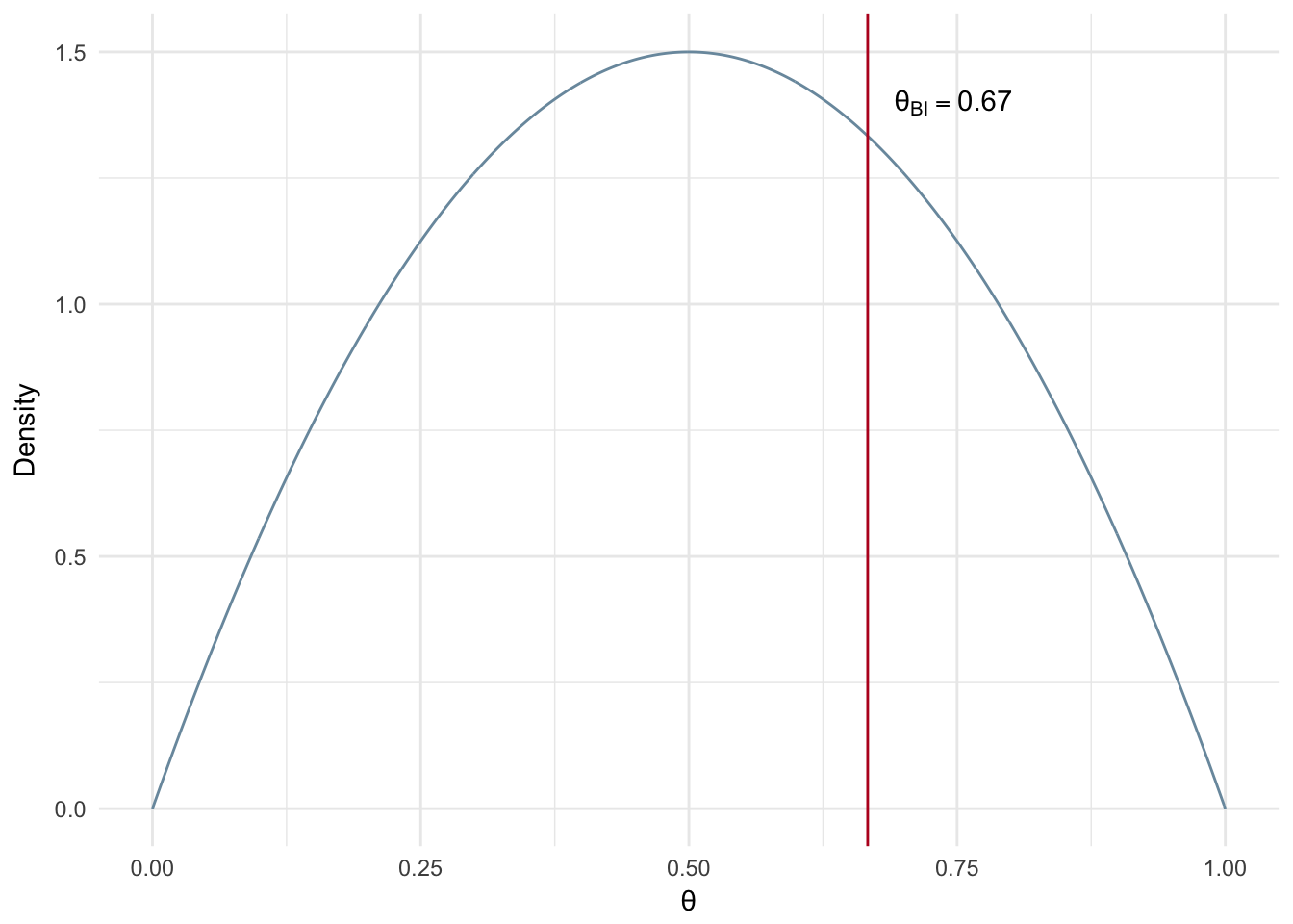

Figure 2.9: Bayesian Inference: Analytical Solution (n=20)

2.6 Gibbs Sampling

The remainder of this chapter will tackle the concept of Gibbs sampling for estimating a posterior distribution. Before getting into specifics let’s touch on why a person may need to use a method such as Gibbs sampling.

2.6.1 The Issue of Intractability

The coin flip example solved via Bayesian inference was capable of being solved analytically. However in many cases of Bayesian inference this is not possible due to the intractability of solving for the marginal likelihood (evidence term). We do have other options for solutions such as Gibbs sampling, expectation-maximization, and Metropolis-Hastings methods. This book will only focus on Gibbs Sampling, but be aware other types of solvers are used for Bayesian inference problems including LDA.

2.6.2 A Tale of Two MC’s

Gibbs Sampling is a Markov Chain Monte Carlo (MCMC) technique for parameter estimation. Let’s break down the two MC’s. A markov chain is a process where the next state is determined by the current state. More importantly it does not rely on any information prior to the current state.

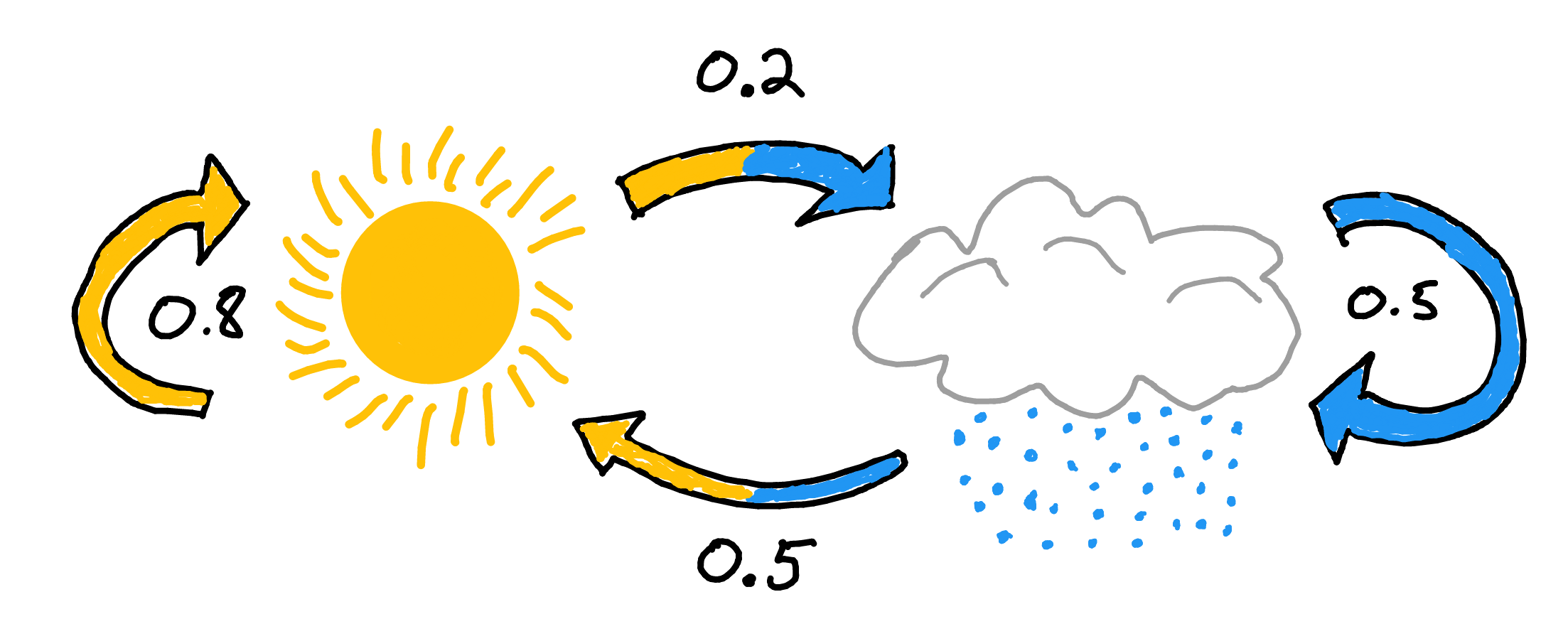
Figure 2.10: Markov Chain: Rain or Shine

The other MC, Monte Carlo, is a technique used to solve a variety of problems by repeated random sampling. A common example used to showcase Monte Carlo methods is the estimation of the value of \(\pi\). (Resnik and Hardisty 2010) All we need is some chalk and a bucket of rice. First I draw a circle on the ground. Then I then draw a square along the circumference of the square. Now for the bucket of rice, aka our random number generator. I stand over the square and uniformly pour rice over the area of the square. Now comes the monotonous part, counting the rice. First I count the number of pieces of rice inside the circle. Next I tally the number of pieces of rice remaining. (Side note: you could save yourself a bunch of time and just weight the two proportions of rice instead of straining your vision and wasting your time.)

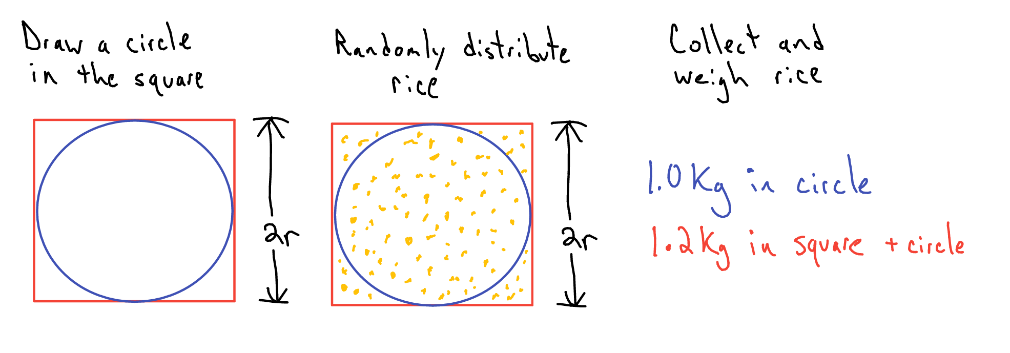
Figure 2.11: Monte Carlo: Estimating π

From here I can infer the value of \(\pi\) as follows:

\[ \begin{equation} \begin{aligned} {\pi r^{2} \over (2r)^{2}} &= {Rice_{circle}\over Rice_{circle + square}} \\\\ \pi &\approx {4Rice_{circle}\over Rice_{circle + square}}\\ \hat{\pi} &= {4*1kg \over 1.2kg} = 3.333 \end{aligned} \tag{2.24} \end{equation} \]

2.6.3 Conjugate Distributions and Priors

Before wading into the deeper water that is Gibbs sampling I need to touch on the concept of conjugate distributions and priors. A conjugate distribution pair is a posterior distribution that have the same form as the prior distribution. Bernoulli and beta distributions are conjugate distributions. The posterior of the bernoulli distribution has the same general form as the prior, the beta distribution. Therefore we call the beta distribution a conjugate prior of the bernoulli distribution. We will cover this specific conjugate relationship in detail in the following section, but you can look ahead at Equations (2.27) (2.28) to see the similar form of the posterior compared to the prior.

Ok, but what does that mean for us? We can use the conjugate relationship to:

1. Simplify our posterior estimation to the same from as the prior.
2. Step 1 allows us to then sample from a known distribution to estimate our posterior distribution.

Step 2 is a crucial component in Gibbs sampling - it is the Monte Carlo piece of the method. To help reinforce the concept of conjugate priors we will go through an example.

2.6.3.1 Bernoulli & Beta

We return to our coin flip example. We want to estimate the posterior, the probability of \(\theta\) given the the results of all experiments (this includes experiments that we haven’t yet completed). Obviously we don’t have data which does not yet exist (i.e. all experiments) so we will need to use the likelihood and the prior to estimate the posterior.

In the previous example we used the Beta distribution for our prior. As we now know, the Beta distribution is the conjugate prior of the Bernoulli distribution. We will take a closer look at this relationship now.

We start with our base relationship between posterior, likelihood, prior, and posterior as shown in Equation (2.25).

\[ \begin{equation} \underbrace{p(\theta|D)}_{posterior} = {\overbrace{p(D|\theta)}^{likelihood} \overbrace{p(\theta)}^{prior} \over \underbrace{p(D)}_{evidence}} \tag{2.25} \end{equation} \]

When estimating the posterior we drop out the evidence term. To reiterate, we can drop out the evidence term because it is constant and is used as a normalizing factor for scaling our probabilities to so that they sum to 1. We will see in the upcoming section that Gibbs sampling accounts for the scaling issue and allows us to infer probabilities at the correct scale.

\[ \begin{equation} \underbrace{p(\theta|D)}_{posterior} \propto {\overbrace{p(D|\theta)}^{likelihood} \overbrace{p(\theta)}^{prior}} \tag{2.26} \end{equation} \]

To estimate the posterior of the bernoulli distribution we plug in our likelihood and prior (Beta distribution) equations in Equation (2.27).

\[ \begin{equation} p(\theta|z,N) \propto \overbrace{\theta^z(1-\theta)^{(N-z)}}^{likelihood} \overbrace{{\theta^{(a-1)}(1-\theta)^{(b-1)}}\over \beta(a,b)}^{prior} \tag{2.27} \end{equation} \]

After combining terms we end up with Equation (2.28) which looks very similar to @(bernBIFinal). This is a very simple example where an analytical solution for the posterior is possible, so the equations are effectively the same with the exeption of the \(\propto\) in place of the \(=\). The \(\propto\) is used because we are going to base our posterior off of random samples from the Beta distribution with the parameters shown in (2.28).

\[ \begin{equation} \begin{aligned} p(\theta|z,N) &\propto {\overbrace{\theta^{(a + z -1)}(1-\theta)^{(N-z+b-1)}}^{Same \hspace{1 mm} Pattern \hspace{1 mm} as \hspace{1 mm} Prior}\over{\beta(a,b)}}\\ p(\theta|z,N) &\propto Beta(a+z, N-z+b) \end{aligned} \tag{2.28} \end{equation} \]

2.6.4 Gibbs Sampling

Gibbs sampling is a Markov Chain Monte Carlo technique that can be used for estimating parameters by walking through a given parameter space. A generalized way to think of Gibbs sampling is estimating a given parameter based on what we currently know about observed data and the other parameters of the model. You may be thinking ‘What other parameters?’. Gibbs sampling is only really applicable when you are trying to estimate multiple parameters otherwise you would use ML, MAP, or analytical Bayesian inference.

Since Gibbs sampling is suited for the estimation of multiple parameters our coin flip example will be expanded slightly. We will now attempt to calculate the bias of two coins and determine if there is a difference in bias between the two using Gibbs sampling.

For the purposes of Gibbs Sampling we need to do a bit of math to determine the equations for our posterior conditional equations. The posterior conditional is the posterior of a single parameter, given the current values of all other parameters in the model. This is where the Markov Chain component of Gibbs sampling comes into play. The conditional posterior of a parameter, i.e. the next state, is determined based on all the current parameter values, i.e. the current state.

Now is a good time to highlight the general structure for using your conjugate priors and how to get to the equations required for the sampling process.

The general process for derivation of our sampling distribution, as outlined in (Yildirim 2012), is as follows:

1. Derive the full joint density.
2. Derive the posterior conditionals for each of the random variables in the model.
3. Simulate samples from the posterior joint distribution based on the posterior conditionals.

So how do we get the posterior conditionals for our two coin problem? First let’s go over what we need to know:

• \(\theta_{1}\) : Bias of coin 1
• \(\theta_{2}\) : Bias of coin 2

The full joint density that defines our problem is shown in Equation (2.29).

\[ \begin{equation} \begin{aligned} p(\theta_{1}, \theta_{2}|z_{1}, z_{2}, N) &\propto p(\theta_{1}|z_{1}, N)p(\theta_{2}|z_{2}, N) \\ p(\theta_{1}, \theta_{2}|z_{1}, z_{2}, N) &\propto p(z_{1}|\theta_{1})p(z_{2}|\theta_{2})p(\theta_{1})p(\theta_{2}) \end{aligned} \tag{2.29} \end{equation} \]

Then we break down the full joint density into our posterior conditionals: \[ \begin{equation} \begin{aligned} p(\theta_{1}|z_{1}, N) &\propto p(z_{1}|\theta_{1})p(\theta_{1}) \\ p(\theta_{2}|z_{2}, N) &\propto p(z_{2}|\theta_{2})p(\theta_{2}) (\#eq:bernFullJointStep2) \end{aligned} \end{equation} \]

We plug in posterior conditional for a single coin, which we derived in Equation (2.28). The resulting posterior conditionals are shown below in Equation (2.30).

\[ \begin{equation} \begin{aligned} p(\theta_{1}|z_{1},N) &\propto Beta(a_{1}+z_{1}, N-z_{1}+b_{1}) \\ p(\theta_{2}|z_{2},N) &\propto Beta(a_{2}+z_{2}, N-z_{2}+b_{2}) \end{aligned} \tag{2.30} \end{equation} \]

Now that we have our posterior conditionals we can move on to estimating our parameters via Gibbs sampling. The general form of Gibbs Sampling is shown in Equation (2.31).

\[ \begin{equation} \begin{aligned} For \ i \ in \ iterations:\\ &p(\theta_{1}^{i+1}) \sim p(\theta_{1}^{i}|\theta_{2}^{i}, \theta_{3}^{i},..., \theta{n}^{i}) \\ &p(\theta_{2}^{i+1}) \sim p(\theta_{2}^{i}|\theta_{1}^{i+1}, \theta_{3}^{i},..., \theta{n}^{i}) \\ &p(\theta_{3}^{i+1}) \sim p(\theta_{3}^{i}|\theta_{1}^{i+1}, \theta_{2}^{i+1},..., \theta{n}^{i}) \\ &................................ \\ &p(\theta_{n}^{i+1}) \sim p(\theta_{n}^{i}|\theta_{1}^{i+1}, \theta_{2}^{i+1},..., \theta_{n-1}^{i+1}) \\ \end{aligned} \tag{2.31} \end{equation} \]

Gibbs sampling works by estimating all parameters via the posterior conditional iteratively for a set number of iterations or a distinct stopping criteria/convergence measure. For the sake of our example we will stick with a set number of iterations. In Equation (2.31) we see the next estimate, i+1, of \(\theta_{1}\) is based on all other current parameter values. When estimating \(\theta_{2}\) the i+1 value of \(\theta_{1}\) is used along with all of the current (i) parameter values. This continues for all parameter values. After the the nth parameter is estimated, the process starts all over again for the next iteration.

The process without the math is shown in Figure 2.12. The red circles represent the parameters yet to be estimated in this iteration where the blue represent those that have been previously estimated during the current iteration. Note that the purple circle in each row is the parameter currently being estimated in that step (the current row) and that it takes into account all the available info, i.e. all the red and blue circles in that row.

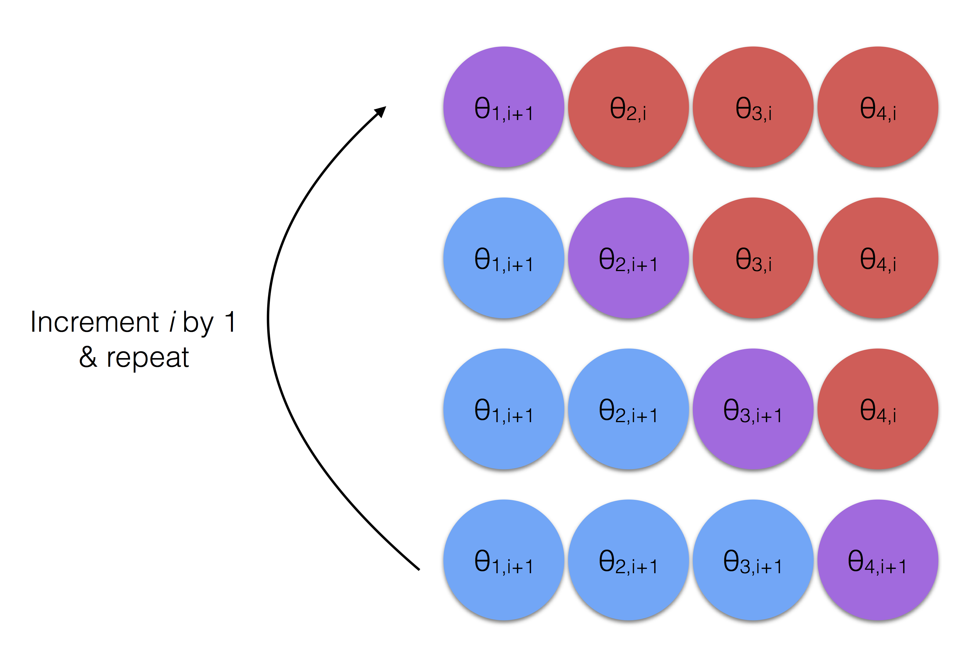
Figure 2.12: Gibbs Sampling - The Process

The calculations used for our example are shown in Equation (2.32). Note that since the two coins are independent of one another, we are sampling from a Beta distribution based on each coin’s priors and evidence then repeating.

\[ \begin{equation} \begin{aligned} For \ i \ in \ iterations:\\ p(\theta_{1}^{i+1}|z_{1},N) &\propto Beta(a_{1}+z_{1}, N-z_{1}+b_{1}) \\ p(\theta_{2}^{i+1}|z_{2},N) &\propto Beta(a_{2}+z_{2}, N-z_{2}+b_{2}) \end{aligned} \tag{2.32} \end{equation} \]

Burn In Period

The purpose of Gibbs Sampling is to sample from the posterior and estimate a parameter value assuming our sampling converges on the true parameter. However it often takes time, i.e. many samples, to move into an area of convergence. To be clear, this is a non-issue for the current example due to the independence between the coins. In the change point example that follows, the parameters are not independent of one another and therefore a burn-in period will be necessary.

2.6.5 Bias of Two Coins

The following example will generate samples from the posterior distributions of two different coins via Gibbs sampling for the purposes of estimating each coin’s bias. We use a fairly weak prior by setting \(\alpha\) and \(\beta\) to a value of 2 for each coins. We have the results of 20 coin flips for each coin. Coin 1 has 10 heads out of 20 flips while coin 2 has 3 heads out of 20 flips.

The Gibbs sampling code below is based on the example provided on Duke’s Computational Statistics and Statistical Computing course website. (Chan and McCarthy 2017)

a = 2
b = 2

z1 = 10
N1 = 20
z2 = 3
N2 = 20


theta = rep(0.5,2)
niters = 10000
burnin = 500

thetas = matrix(0, nrow = (niters-burnin), ncol=2)
for (i in 1:niters){

  theta1 = rbeta(n = 1, shape1 = a + z1, shape2 = b + N1 - z1)
  # get value theta2| all other vars
  theta2 = rbeta(n = 1, shape1 = a + z2, shape2 =b + N2 - z2)
  
  if (i >= burnin){
    thetas[(i-burnin), ] = c(theta1, theta2)
  }
}


ds <- data.frame(theta1 = thetas[,1], theta2= thetas[,2])
ggplot(ds, aes(x=theta1)) + geom_histogram(aes(y=..density..),color='#1A384A', fill='#7A99AC') + 
  labs(title = expression(theta[1]~Estimate), x=expression(theta[1]), y = 'Density') + 
  geom_vline(xintercept = mean(ds$theta1), color='#b7091a') +
  theme_minimal()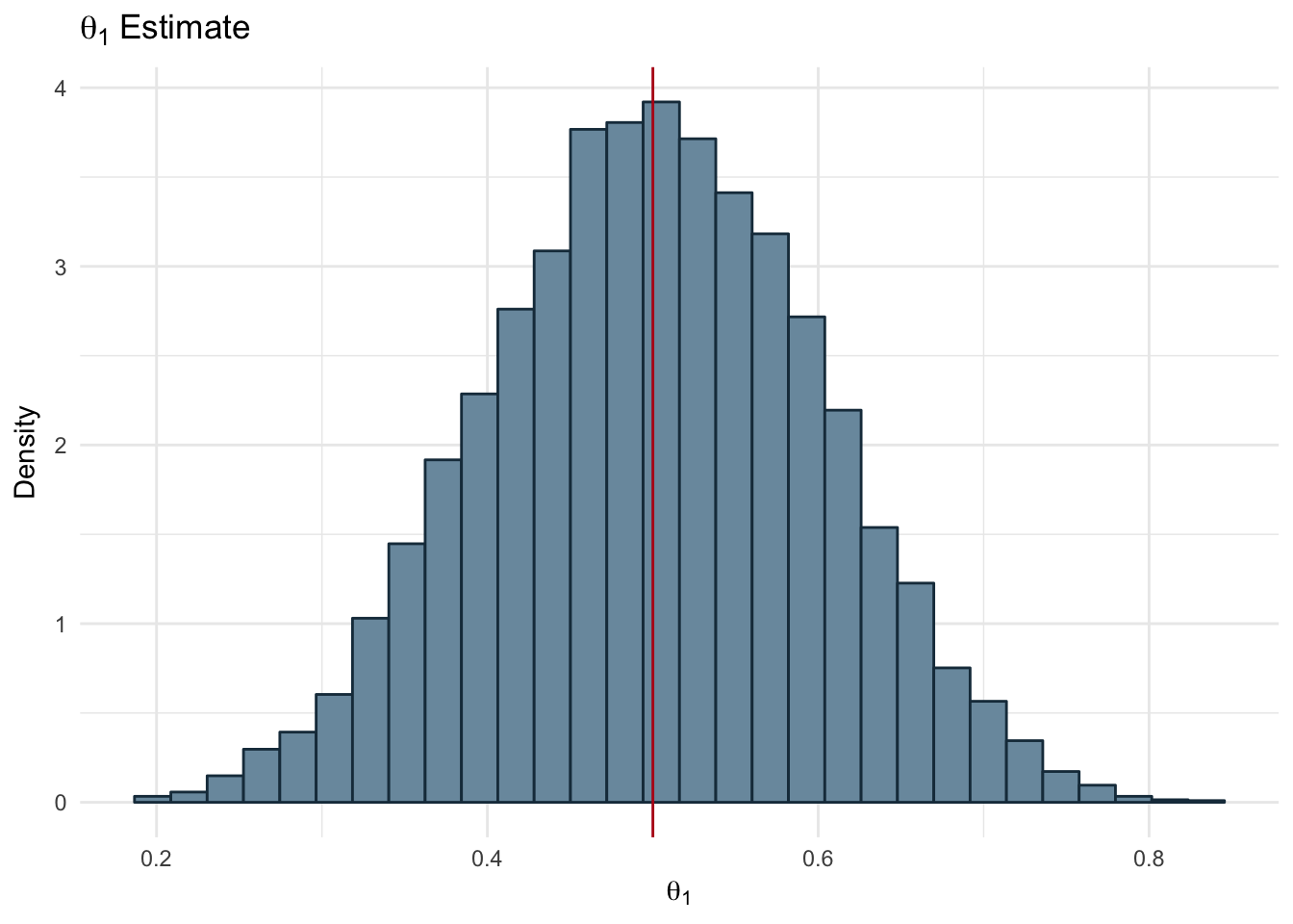

Figure 2.13: Bias of Two Coins: Theta 1

ggplot(ds, aes(x=theta2)) + geom_histogram(aes(y=..density..),color='#1A384A', fill='#7A99AC') + 
  labs(title = expression(theta[2]~Estimate), x=expression(theta[2]), y = 'Density') + 
  geom_vline(xintercept = mean(ds$theta2), color='#b7091a') + 
  theme_minimal()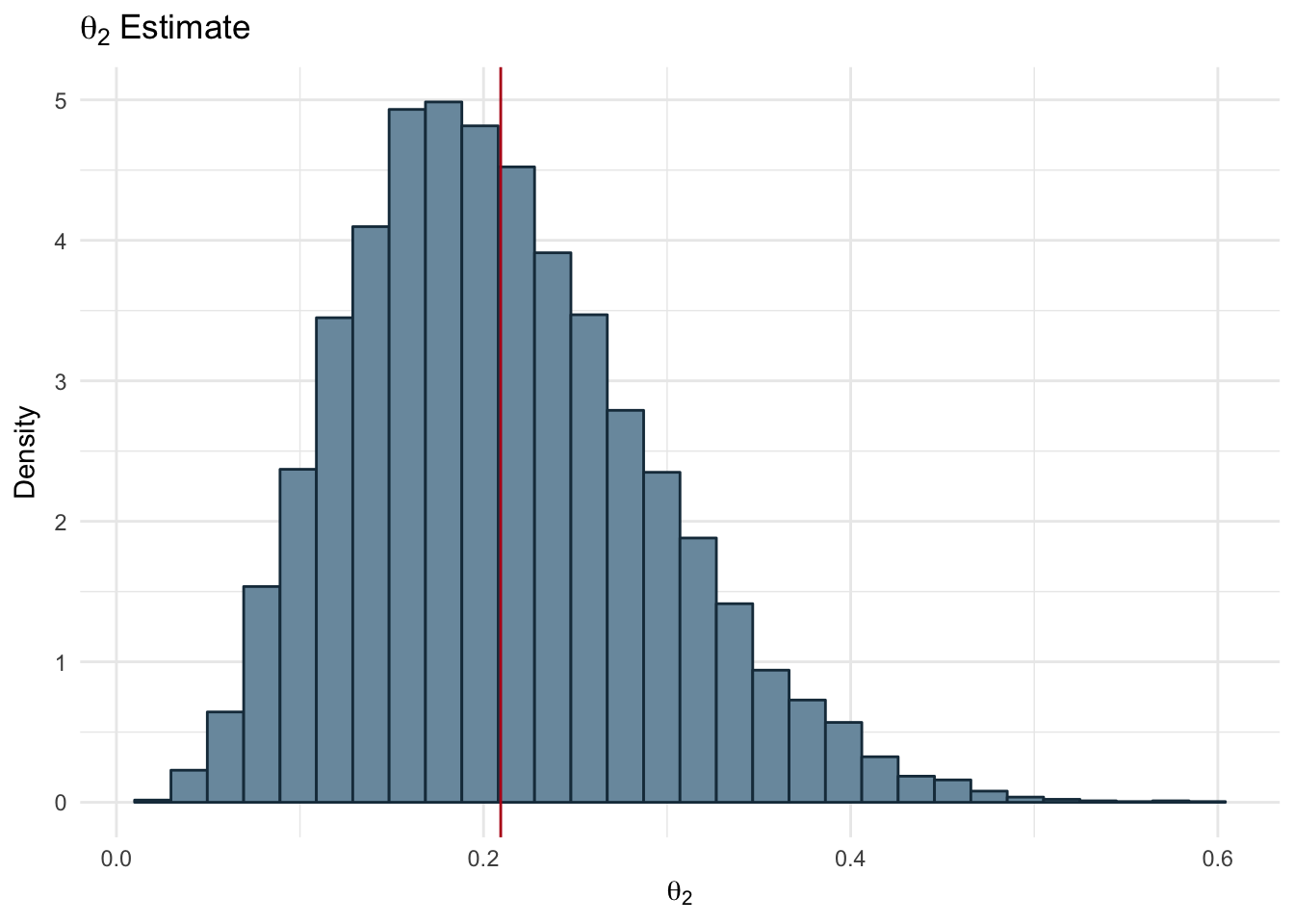

Figure 2.14: Bias of Two Coins - Theta 2

In the Figures 2.14 and 2.13 we can see the distribution of samples drawn from the Beta distribution using the prior parameters and the observed data we have. The red line represents the mean of the samples for each coin. Our resulting bias values are:

• \(\theta_{1}\) = 0.5
• \(\theta_{2}\) = 0.21

2.6.6 Change Point Example

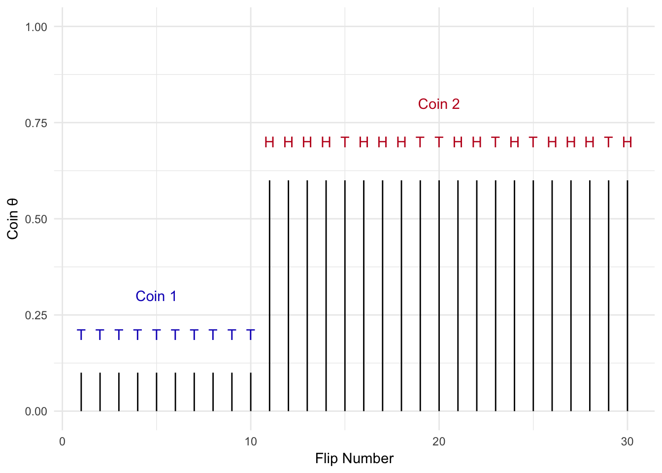
Figure 2.15: Change Point Example

What if the problem we are solving is more complicated? Let’s say I flip a coin repeatedly, but at some point I switch to another coin with a different bias (\(\theta\)) as shown in Figure 2.15. I want to detect the point in time when coin 1 was swapped out for coin 2. We can use Gibbs sampling to solve this problem.

In the previous example we only needed to get a posterior of a single variable (technically there were two variables, but both have the same posterior conditional and were independent of one another). In this case we have 3 variables that we need to estimate:

1. Coin bias for coin 1: \(\theta_{1}\)
2. Coin bias for coin 2: \(\theta_{2}\)
3. The point in time, i.e. on which flip, the coin was swapped from coin 1 to coin 2: n

We have three variables, but how do we describe the actual process we are modeling? In Equation (2.33) the distrutions for each variable are displayed. The coinflips, x, are drawn from a bernoulli distribution, but are dependent on the coin being flipped and the bias of that coin, \(\theta_{i}\). From the previous examples we know \(\theta\) is modeled using a beta distribution. The change point, n, is the time when coin 2 replaces coin 1. Therefore the possible values of n are between 2, the second sample in discrete time, and N, the final discrete time in our example. All values of n are equally probable and therefore can be modeled as a uniform distribution.

\[ \begin{equation} \begin{aligned} x &\sim \begin{cases} Bern(x_{i};\theta_{1}) \quad 1 \le i \le n \\ Bern(x_{i};\theta_{2}) \quad n \lt i \lt N \end{cases} \\ n &\sim Uniform(2...N) \\ \theta_{i} &\sim Beta(\theta_{i}, a,b) \end{aligned} \tag{2.33} \end{equation} \]

2.6.6.1 Derivation of Joint Distribution

Now that we have defined all the unknowns of our model, we derive the full joint distribution.

\[ \begin{equation} p(\theta_{1}, \theta_{2}, n| x_{1:n}) \propto \overbrace{p(x_{1:N}|\theta_{1}) p(x_{n+1:N}|\theta_{2})}^{Likelihoods} \overbrace{p(\theta_{1})p(\theta_{2})p(n)}^{Priors} \tag{2.34} \end{equation} \]

Our goal here is to get one equation to estimate the posterior of each of our variables, aka the posterior conditionals. The easiest way to accomplish this task is to identify the terms of the joint distribution that contain the variable you want the posterior conditional for.

Let’s start by breaking (2.34) a bit further.

$$ \[\begin{equation} \begin{aligned} p(\theta_{1}, \theta_{2}, n| x_{1:n}) &\propto (\prod_{1}^{n}p(x_{i}|\theta_{1})) (\prod_{n+1}^{N}p(x_{i}|\theta_{2})) p(\theta_{1})p(\theta_{2})p(n)\\ &\propto [\theta_{1}^{z_{1}}(1-\theta_{1})^{n-z_{1}}] [\theta_{2}^{z_{2}}(1-\theta_{2})^{N-(n+1)-z_{2}}] p(\theta_{1})p(\theta_{2})p(n)\\ \\ &\propto [\theta_{1}^{z_{1}}(1-\theta_{1})^{n-z_{1}}] [\theta_{2}^{z_{2}}(1-\theta_{2})^{N-(n+1)-z_{2}}] {{\theta_{1}^{(a_{1}-1)}(1-\theta_{1})^{(b_{1}-1)}}\over \beta(a_{1},b_{1})} {{\theta_{2}^{(a_{2}-1)}(1-\theta_{2})^{(b_{2}-1)}}\over \beta(a_{2},b_{2})} {1\over N}\\ \\ \end{aligned} \tag{2.35} \end{equation}\]

$$

Then we move on to solving for n’s posterior conditional. In Equation (2.35) we see that only the likelihood terms and the priors for the \(\theta\)’s contain n. Using these terms we can solve for the posterior conditional. While we are at it we will also take the log of the conditional posterior as is good practice to prevent issues such as underflow.

\[ \begin{equation} \begin{aligned} p(n| x_{1:n}, \theta_{1}, \theta_{2}) &\propto [\theta_{1}^{z_{1}}(1-\theta_{1})^{n-z_{1}}] [\theta_{2}^{z_{2}}(1-\theta_{2})^{N-(n+1)-z_{2}}]\\ log(p(n| x_{1:n}, \theta_{1}, \theta_{2})) &\propto log([\theta_{1}^{z_{1}}(1-\theta_{1})^{n-z_{1}}]) + log([\theta_{2}^{z_{2}}(1-\theta_{2})^{N-(n+1)-z_{2}}]) \end{aligned} \end{equation} \]

To get the posterior conditionals for the \(\theta\) values we will need to utilize the conjugate prior relationship between the likelihoods and the priors. First we will collapse the priors and likelihoods for the \(\theta\) values.

\[ \begin{equation} \begin{aligned} p(\theta_{1}, \theta_{2}, n| x_{1:n}) &\propto [\theta_{1}^{(z_{1}+a_{1}-1)}(1-\theta_{1})^{(n-z_{1}+b_{1}-1)}] [\theta_{2}^{(z_{2}+a_{2}-1)}(1-\theta_{2})^{(N-n-1-z_{2}+b_{2}-1)}]({1 \over N})\\ &\propto Beta(a_{1}+z_{1}, n-z_{1}+b_{1}) Beta(z_{2}+a_{2}, N-n-1-z_{2}+b_{2})({1\over N}) \end{aligned} \end{equation} \]

Now we can solve for each of the \(\theta\)’s posterior conditionals.

\[ \begin{equation} \begin{aligned} p(\theta_{1}| x_{1:n},\theta_{2}, n) &\propto Beta(a_{1}+z_{1}, n-z_{1}+b_{1})\\ log(p(\theta_{1}| x_{1:n},\theta_{2}, n)) &\propto log(Beta(a_{1}+z_{1}, n-z_{1}+b_{1})) \end{aligned} \end{equation} \]

\[ \begin{equation} \begin{aligned} p(\theta_{2}| x_{1:n},\theta_{1}, n) &\propto Beta(z_{2}+a_{2}, N-n-1-z_{2}+b_{2})\\ log(p(\theta_{2}| x_{1:n},\theta_{1}, n)) &\propto log(Beta(z_{2}+a_{2}, N-n-1-z_{2}+b_{2})) \end{aligned} \end{equation} \]

Now let’s put our derived posteriors to work use Gibbs sampling to estimate our change point and coin biases.

real_thetas <- c(0.2, 0.6)
N <- 300
a = 2
b = 3
change_point <- 100
x <- c(rbinom(1:change_point, 1, real_thetas[1]),rbinom((change_point+1):N, 1, real_thetas[2]))


## Initialize all parameters

# n ~ uniform 
n <- round(N*runif(1))
# theta1 ~ beta(a,b)
theta1 <- rbeta(1, a, b)
# theta2 ~ beta(a,b)
theta2 <- rbeta(1, a, b)



niters = 3000
burnin = 1000

params = matrix(0, nrow = (niters-burnin), ncol=3)
for (i in 1:niters){
  
  
  z1 <- sum(x[1:n])
  if(n == N){
    z2 <- 0
  }else{
    z2 <- sum(x[(n+1):N])
  }
  theta1 = rbeta(n = 1, shape1 = a + z1, shape2 = b + n - z1)
  # get value theta2| all other vars
  theta2 = rbeta(n = 1, shape1 = a + z2, shape2 =N-n-1-z2+b)
  
  
  ## 2 things: 1 - should I be summing all the values over these? 
  # No - the product is being calculated due to the sum - should be fine
  n_multi <- rep(0, N)
  for(steps in 2:N){
    if(steps==N || theta2 == 1){
      n_multi[steps] <- log(theta1^sum(x[1:steps]) * (1-theta1)^(steps-sum(x[1:steps])))
    }else{
      n_multi[steps] <- log(theta1^sum(x[1:steps]) * (1-theta1)^(steps-sum(x[1:steps]))) +
        log(theta2^sum(x[(steps + 1):N]) * (1-theta2)^(N-steps-1-sum(x[(steps+1):N])))
    }
  }
  
  n_multi <- exp(n_multi[2:N] - max(n_multi[2:N]))
  # offset by 1 
  # you n is equally probably between 2 and N and zero at n=1
  # we only calculate p(n) from n=2 to N
  n <- which(rmultinom(1, 1, n_multi/sum(n_multi))[,1] ==1) + 1
  if (i >= burnin){
    params[(i-burnin), ] = c(theta1,theta2, n)
  }
}

ds <- data.frame(x = x, theta = c(rep(real_thetas[1],N-change_point),
                                  rep(real_thetas[2],change_point)), 
                 sample_index = seq(1:length(x)))

params_df <- as.data.frame(params)
names(params_df) <- c('theta1', 'theta2', 'change_point')

ggplot(params_df, aes(x = change_point)) + 
  geom_histogram(fill="#7A99AC", color ='#1A384A', binwidth = 5, bins = floor(N/5)) +
  theme_minimal() + 
  scale_x_continuous(limits = c(0,N)) +
  geom_vline(xintercept = mean(params_df$change_point), color='#b7091a') +
  labs(title = 'Change Point Estimate', x='Change Point', y = 'Density') 

Figure 2.16: Estimated Change Point

ggplot(params_df, aes(x = theta1)) + 
  geom_histogram(fill="#7A99AC", color ='#1A384A' , binwidth = 0.025) + 
  theme_minimal() + 
  scale_x_continuous(limits = c(0,1)) +
  geom_vline(xintercept = mean(params_df$theta1), color='#b7091a') +
  labs(title = expression(theta[1]~Estimate), x=expression(theta[1]), y = 'Density')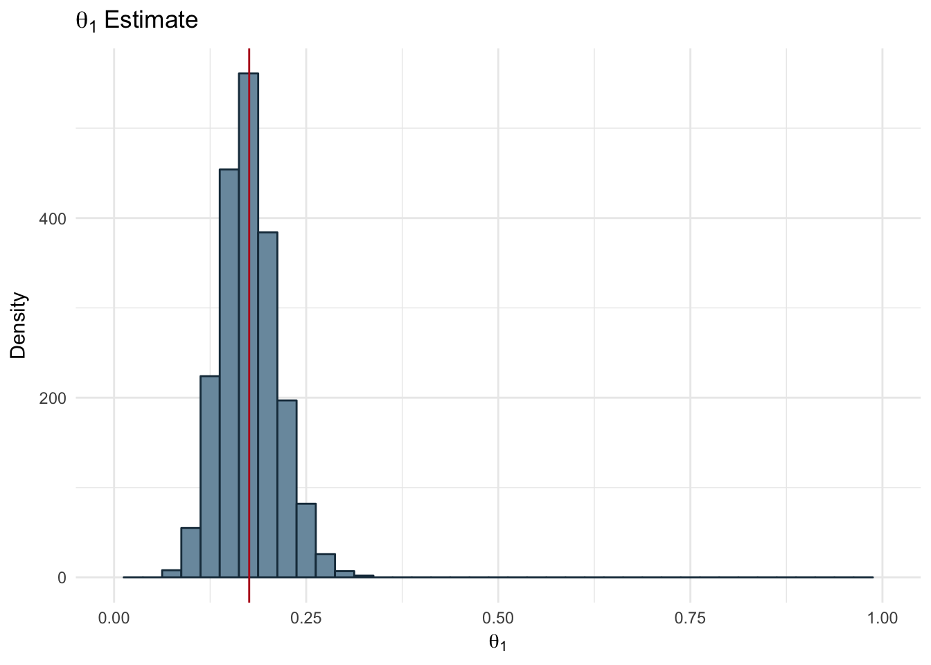 

Figure 2.17: Estimated Theta 1

ggplot(params_df, aes(x = theta2)) + 
  geom_histogram(fill="#7A99AC", color ='#1A384A' , binwidth = 0.025) + 
  theme_minimal() + 
  scale_x_continuous(limits = c(0,1)) +
  geom_vline(xintercept = mean(params_df$theta2), color='#b7091a') +
  labs(title = expression(theta[2]~Estimate), x=expression(theta[2]), y = 'Density')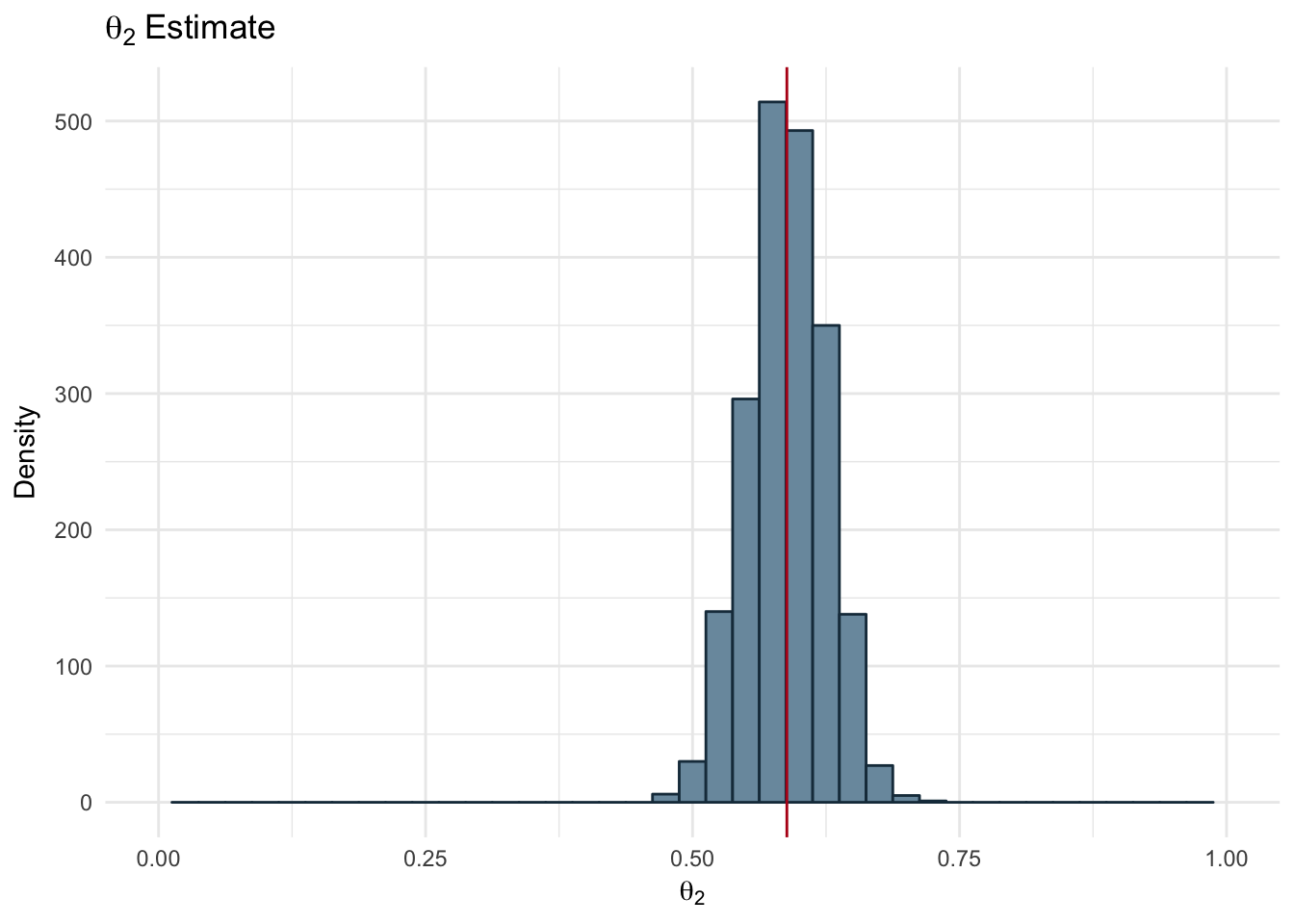 

Figure 2.18: Estimated Theta 2

The resulting estimates for each of our parameters is shown below along with the real value used to generate the dataset.

data.frame(theta_1 = c(real_thetas[1], mean(params_df$theta1)),
       theta_2 = c(real_thetas[2], mean(params_df$theta2)),
       n = c(change_point, floor(mean(params_df$change_point))),
       row.names = c('True', 'Estimated')) %>% 
  kable(col.names = c('\u03b8\u2081', '\u03b8\u2082', 'n'),
        digits = 2,
        row.names = TRUE, 
        caption = 'Change Point Parameters and Estimates')

Table 2.1: Change Point Parameters and Estimates

	θ₁	θ₂	n
True	0.20	0.60	100
Estimated	0.18	0.59	101