1 What is LDA?
Latent Dirichlet Allocation (LDA) is a generative probablistic model for collections of discrete data developed by Blei, Ng, and Jordan. (Blei, Ng, and Jordan 2003) The most common use of LDA is for modeling of collections of text, also known as topic modeling.
A topic is a probability distribution over words.(Steyvers and Griffiths 2007) Imagine you have a bag that has a bunch of little squares in it with a word printed on each (similar to the game Scrabble, but a word on each chip instead of a single letter). Any word not in the bag has a probability of being drawn equal to zero. However, all other words in the bag have a probability greater than zero. Let’s say we have 2 chips with the word ‘Philadelphia’ and 1 with the word ‘Eagles’ on it. We would say you have a 1/3 chance of drawing ‘Eagles’, 2/3 chance of drawing ‘Philadelphia’, and 0 for any other word. This is effectively what a topic is; it provides us with the probabilities of a set of words for the given topic.
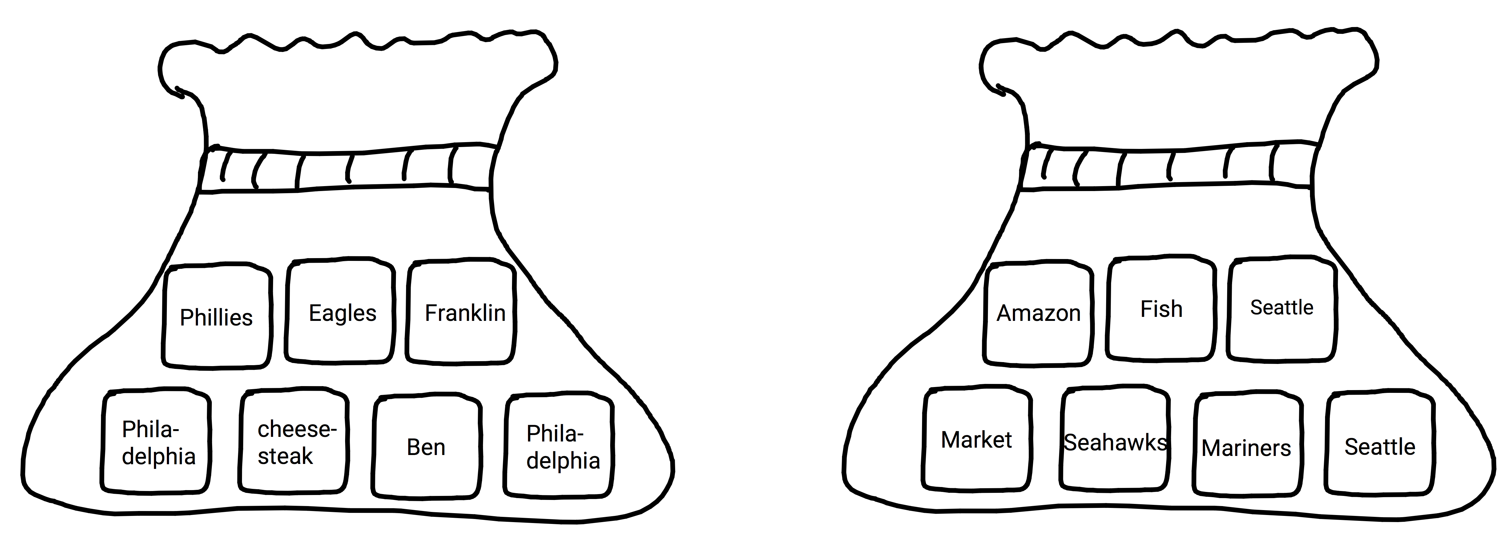
Figure 1.1: Topic Scrabble: Philadelphia and Seattle
The general idea of LDA is that each document is generated from a mixture of topics and each of those topics is a mixture of words. This can be used as a mechanism for generating new documents, i.e. we know the topics a priori, or for inferring topics present in a set of documents we already have.
In regards to the model name, you can think of it as follows:
- Latent: Topic structures in a document are latent meaning they are hidden structures in the text.
- Dirichlet: The Dirichlet distribution determines the mixture proportions of the topics in the documents and the words in each topic.
- Allocation: Allocation of words to a given topic.
To review: we have latent structures in a corpus (topics), with topic distributions in each document and word distributions in each topic based on the Dirichlet distribution, to allocate words to a given topic and topics to a given document.
I realize some readers may be unfamiliar with a portion of the terminology and distributions mentioned in the opening paragraphs. Please keep reading, all the nuts an bolts will be addressed in the following chapters, but to help get an understanding of what LDA is and why it is useful, I will offer a quick example. We will get to the math and technical concepts in the following chapters.
1.1 Animal Generator
The majority of this book is about words, topics, and documents, but lets start with something a bit different: animals and where they live. One of the ways you can classify animals is by where they spend the majority of their time - land, air, sea. Obviously there are some animals that only dwell in one place; a cow only lives on land and a fish only lives in the sea. However, there are other animals, such as some birds, that split their time between land, sea, and air.
You are probably asking yourself ‘where is he going with this?’. We can think of land, air, and sea as topics that contain a distribution of animals. In this case we can equate animals with words. For example, on land I am much more likely to see a cow than a whale, but in the sea it would be the reverse. If I quantify these probabilities into a distribution over all the animals (words) for each type of habitat (land,sea, air - topics) I can use them to generate sets of animals (words) to populate a given location (document) which may contain a mix of land, sea, and air (topics).
So let’s move on to generating a specific location. We know that different locations will vary in terms of which habitats are present. For example, a beach contains land, sea, and air, but some areas inland may only contain air and land like a desert. We can define the mixture of these types of habitats in each location. For example, a beach is 1/3 land, 1/3 sea, and 1/3 air. We can think of the beach as a single document. To review: a given location (document) contains a mixture of land, air, and sea (topics) and each of those contain different mixtures of animals (words).
Let’s work through some examples using our animals and habitats. The examples provided in this chapter are oversimplified so that we can get a general idea how LDA works.
We’ll start by generating our beach location with 1/3 land animals, 1/3 sea animals, and 1/3 air animals. Below you can see our collection of animals and their probability in each topic. Note that some animals have zero probabilities in a given topic, i.e. a cow is never in the ocean, where some have higher probabilities than others; a crab is in the sea sometimes, but a fish is always in the sea. You may notice that there is only 1 animal in the air category. There are several birds, but only 1 of them is cabable of flight in our vocabulary.
| vocab | land | sea | air |
|---|---|---|---|
| 🐋 | 0.00 | 0.12 | 0 |
| 🐳 | 0.00 | 0.12 | 0 |
| 🐟 | 0.00 | 0.12 | 0 |
| 🐠 | 0.00 | 0.12 | 0 |
| 🐙 | 0.00 | 0.12 | 0 |
| 🦀 | 0.05 | 0.06 | 0 |
| 🐊 | 0.05 | 0.06 | 0 |
| 🐢 | 0.05 | 0.06 | 0 |
| 🐍 | 0.05 | 0.06 | 0 |
| 🐓 | 0.10 | 0.00 | 0 |
| 🦃 | 0.10 | 0.00 | 0 |
| 🐦 | 0.05 | 0.06 | 1 |
| 🐧 | 0.05 | 0.06 | 0 |
| 🐿 | 0.10 | 0.00 | 0 |
| 🐘 | 0.10 | 0.00 | 0 |
| 🐂 | 0.10 | 0.00 | 0 |
| 🐑 | 0.10 | 0.00 | 0 |
| 🐪 | 0.10 | 0.00 | 0 |
To generate a beach (document) based off the description we would use those probabilities in a straightforward manner:
words_per_topic <- 3
equal_doc <- c(vocab[sample.int(length(vocab),words_per_topic, prob=phi_ds$land, replace = T)],
               vocab[sample.int(length(vocab),words_per_topic, prob=phi_ds$sea, replace = T)],
               vocab[sample.int(length(vocab),words_per_topic, prob=phi_ds$air, replace = T)])
cat(equal_doc)
## 🐘 🐂 🐪 🐧 🐧 🐙 🐦 🐦 🐦In the above example the topic mixtures are static and equal, so each habitat (topic) contributes 3 animals to the beach.
Before proceeding, I want to take a moment to give recognition to Tim Hopper for his presentation utilizing emoji to shed some light on how generative LDA works (Hopper 2016).
Ok, now let’s make an ocean setting. In the case of the ocean we only have sea and air present, so our topic distribution in the document would be 50% sea, 50% air, and 0% land.
words_per_topic <- 3
ocean_doc <- c(vocab[sample.int(length(vocab),words_per_topic, prob=phi_ds$sea, replace = T)],
               vocab[sample.int(length(vocab),words_per_topic, prob=phi_ds$air, replace = T)])
cat(ocean_doc)
## 🐋 🐳 🐢 🐦 🐦 🐦In the example above only the air and land contribute to the ocean location. Therefore they both contribute an equal number of animals to the location.
1.1.1 Generating the Mixtures
It is important to note the examples above use static word and topic mixtures that were predetermined, but these mixtures could just as easily be created by sampling from a Dirichlet distribution. This is an important distinction to make as it is the foundation of how we can use LDA to infer topic structures in our documents. The Dirichlet distribution and it’s role in LDA is discussed in detail in the coming chapters.
1.2 Inference
We have seen that we can generate collections of animals that are representative of the given location. What if we have thousands of locations and we want to know the mixture of land, air, and sea that are present? And what if we had no idea where each animal spends its time? LDA allows us to infer both of these peices of information. Similar to the locations (documents) generated above, I will create 100 random documents with varying length and various habitat mixtures.
| Document | Animals |
|---|---|
| 1 | 🐪 🐘 🐪 🐘 🐦 🐓 🐪 🐪 🐍 🐪 🐧 🦀 🦀 🐪 🐓 🐍 🐘 🐓 🐍 🐿 🐧 🐢 🐧 🦃 🦃 🐧 🐦 🐑 🐑 🐊 🐳 🦀 🦀 🐿 🐢 🐢 🐿 🐓 🐪 🐊 🐘 🐦 🐪 🐂 🐍 🐓 🐍 🐓 🐦 🐍 🦃 🐦 🐪 🐍 🐿 🐦 🐦 🐂 🐿 🐍 🐂 🐿 🐦 🐦 🐑 🐂 🐓 🐓 🐧 🐑 🐦 🐪 🐦 🐧 🐿 🐪 🐦 🐢 🦃 🐿 🦃 🐦 🐑 🐊 🦃 🐪 🦃 🐓 🐂 🐊 🐊 🐂 🦃 |
| 2 | 🐙 🐂 🐦 🐦 🐓 🐧 🐪 🐙 🐧 🐙 🐪 🐘 🐋 🐂 🐦 🐧 🐦 🐙 🐦 🐳 🐟 🐊 🐟 🐢 🐠 🐠 🐪 🐢 🐦 🐘 🐍 🐳 🦃 🐟 🐙 🦀 🐊 🐳 🐪 🐠 🐧 🐢 🐢 🐦 🐍 🐧 🐿 🐢 🐪 🐢 🐧 🐓 🐑 🐳 🐧 🐍 🐊 🐂 🦃 🐋 🐪 🐓 🐿 🐟 🐙 🐋 🦀 🐂 🐦 🐳 🐢 🐟 🐦 🐘 🐊 🐓 🐓 🐧 🐊 🐢 🐪 🐓 🐊 🐢 🐑 🐢 🐙 🐊 🐢 🐧 🐪 |
The topic word distributions shown in Table 1.1 were used to generate our sample documents. The true habitat (topic) mixtures used to generate the first couple of documents are shown in Table 1.3:
| Document | air | land | sea |
|---|---|---|---|
| 1 | 0.09 | 0.90 | 0.01 |
| 2 | 0.09 | 0.51 | 0.39 |
With the help of LDA we can go through all of our documents and estimate the topic/word (habitat/animal) distributions and the topic/document (habitat/location) distributions.
The true and estimated topic word distributions are shown in Table 1.4.
| air estimated | air | land estimated | land | sea estimated | sea | |
|---|---|---|---|---|---|---|
| 🐋 | 0.00 | 0 | 0.00 | 0.00 | 0.11 | 0.12 |
| 🐳 | 0.01 | 0 | 0.01 | 0.00 | 0.10 | 0.12 |
| 🐟 | 0.00 | 0 | 0.00 | 0.00 | 0.11 | 0.12 |
| 🐠 | 0.00 | 0 | 0.00 | 0.00 | 0.12 | 0.12 |
| 🐙 | 0.00 | 0 | 0.00 | 0.00 | 0.12 | 0.12 |
| 🦀 | 0.01 | 0 | 0.04 | 0.05 | 0.06 | 0.06 |
| 🐊 | 0.00 | 0 | 0.05 | 0.05 | 0.07 | 0.06 |
| 🐢 | 0.01 | 0 | 0.05 | 0.05 | 0.06 | 0.06 |
| 🐍 | 0.00 | 0 | 0.06 | 0.05 | 0.05 | 0.06 |
| 🐓 | 0.00 | 0 | 0.10 | 0.10 | 0.00 | 0.00 |
| 🦃 | 0.00 | 0 | 0.10 | 0.10 | 0.00 | 0.00 |
| 🐦 | 0.95 | 1 | 0.02 | 0.05 | 0.11 | 0.06 |
| 🐧 | 0.00 | 0 | 0.05 | 0.05 | 0.06 | 0.06 |
| 🐿 | 0.00 | 0 | 0.10 | 0.10 | 0.01 | 0.00 |
| 🐘 | 0.00 | 0 | 0.10 | 0.10 | 0.00 | 0.00 |
| 🐂 | 0.00 | 0 | 0.10 | 0.10 | 0.00 | 0.00 |
| 🐑 | 0.00 | 0 | 0.10 | 0.10 | 0.01 | 0.00 |
| 🐪 | 0.00 | 0 | 0.11 | 0.10 | 0.00 | 0.00 |
The document topic mixtures and the estimated mixtures are shown below for the first 5 documents:
| Location | air estimated | air | land estimated | land | sea estimated | sea |
|---|---|---|---|---|---|---|
| 1 | 0.09 | 0.09 | 0.90 | 0.90 | 0.01 | 0.01 |
| 2 | 0.05 | 0.09 | 0.46 | 0.51 | 0.48 | 0.39 |
| 3 | 0.41 | 0.36 | 0.54 | 0.64 | 0.05 | 0.00 |
| 4 | 0.53 | 0.50 | 0.45 | 0.48 | 0.02 | 0.01 |
| 5 | 0.47 | 0.41 | 0.25 | 0.40 | 0.27 | 0.19 |
| 6 | 0.03 | 0.02 | 0.35 | 0.38 | 0.62 | 0.59 |
The results of our estimations of both the word topic distributions and the document topic distributions have some variation from the true distributions used to generate the documents. The cosine similarity between the estimated and true topic proportions in each document are shown below.
| air | land | sea |
|---|---|---|
| 0.99 | 0.99 | 0.99 |
| air | land | sea |
|---|---|---|
| 1.00 | 0.99 | 0.98 |